SUMPRODUCT in Excel

What is SUMPRODUCT in Excel?

The SUMPRODUCT function in Excel finds the product of the corresponding values in the arrays specified and returns its sum. Thus, it can help calculate and compare numbers in two or more ranges. Therefore, if you need to find both the product and the sum of arrays or corresponding ranges, you can use the SUMPRODUCT. It is classified under Math and Trigonometric functions.

For instance, you purchase some items in a shop and need the final bill to pay your amount. First, let us look at how SUMPRODUCT calculates it. To find the total billing amount, you must multiply the price of each item and the number of items bought and, finally, get the sum. To find the billing amount, we use the formula =SUMPRODUCT(C2:C5, D2:D5) in cell D7.

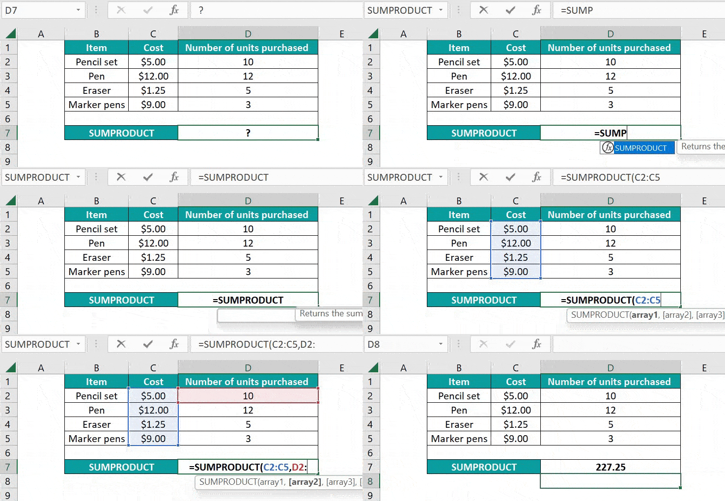
With the help of this function, you can obtain both the sum and product of the chosen arrays in a single cell.

What is SUMPRODUCT in Excel?

The function SUMPRODUCT in Excel returns the sum of the products of corresponding arrays or ranges specified in the function. Besides multiplication, you can also perform addition, subtraction, and division.
For this, you must replace the commas which separate the ranges in the function with (+,-,*,/). It can accept up to 255 arguments. At least one array argument is mandatory.
SUMPRODUCT performs the operations of other functions and can be used to write complex formulas. It can be used with COUNTIF, LEN, VLOOKUP, MOD, etc.

SUMPRODUCT() Excel Function

The syntax for SUMPRODUCT in Excel is as follows:

Arguments:

array1 (mandatory): This specifies the first range to multiply and then add
[array2], [array3] …(optional): If provided, these arrays will also be multiplied and then added. You can specify up to 255 arrays.

In case only a single array/range is provided, it sums the elements in the array. In the case of multiple ranges, though it’s an array Excel formula, pressing Enter is enough, and you do not have to press Ctrl + Shift + Enter.

Excel VBA – All in One Courses Bundle (35+ Hours of Video Tutorials)

If you want to learn Excel and VBA professionally, then Excel VBA All in One Courses Bundle (35+ hours) is the perfect solution. Whether you’re a beginner or an experienced user, this bundle covers it all – from Basic Excel to Advanced Excel, Macros, Power Query, and VBA.

Start Learning Now

How to Use SUMPRODUCT Excel Function?

We can use the SUMPRODUCT Excel function in two ways. It can be entered as a part of a formula in an Excel cell, or we can access it from the Excel ribbon.

Entering SUMPRODUCT in Excel Manually

The SUMPRODUCT function can be entered manually in a cell to obtain the sales made by a particular individual. For example, the sales details of a few employees are in the table below.

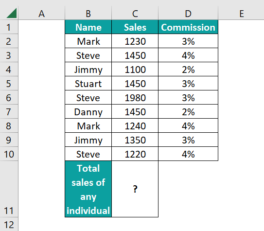
How to use SUMPRODUCT Excel Function - Basic Example

The total sales of a particular employee can be obtained by entering the following formula in cell C11.
=SUMPRODUCT((C2:C10*D2:D10)*(B2:B10=”Steve”))
• Here, we take the values in Column D, the commission percentages, and use them against the sales data in Column C to find the commission received by an employee called Steve.
• Using the conditional operator “=”, we can find the commission received by a particular employee.
• You can substitute any desired operators (*, /, +, -) in place of commas separating the ranges to perform different functions, like we have used ‘*’ here.

Thus, the SUMPRODUCT function can find the sum and product of specific values in a range for a particular entity.

Entering SUMPRODUCT through the Excel Ribbon

Besides manually entering the formula, you can also use the SUMPRODUCT excel function shortcut through the Excel ribbon.

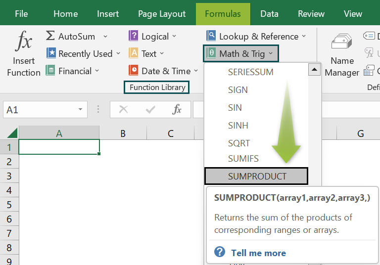
Step 1: Place the cursor where you want the formula to be entered. Then, in the Excel ribbon, go to the Formulas tab and click on the Math & Trig drop-down arrow in the Function Library group.

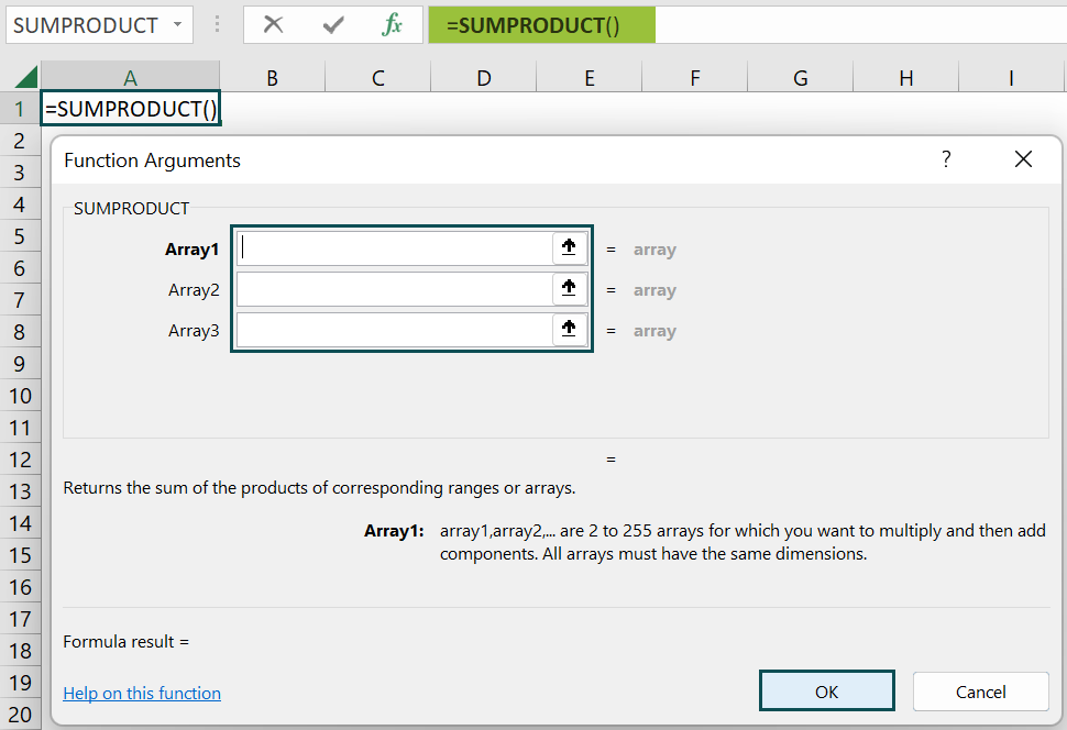
How to use SUMPRODUCT Excel Function - Enter through the Excel ribbon

Step 2: Once you select the SUMPRODUCT function, you get a dialog window. Enter the values for the required number of arrays. Note that one array is mandatory. Then, you get the result in the cell where the cursor is placed.

How to use SUMPRODUCT Excel Function - Function arguments window

Thus, we can enter the formula in different ways for calculations. But first, let us look at the examples below to see how we can implement the function in various real-time scenarios.

Examples

Here are some examples to understand how you can use SUMPRODUCT to find many different types of values.

Example #1

You can use SUMPRODUCT in Excel with condition to find certain values. For example, consider a list of products purchased by a businessman. Suppose he wants to find the number of times he has purchased a particular product. We can use the SUMPRODUCT under such conditions.

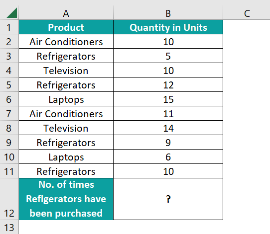
Step 1: Let us find out the number of times he has purchased refrigerators. For this, you need to apply the following formula in cell B12.

=SUMPRODUCT(–(A2:A11=”Refrigerators”))

The SUMPRODUCT searches the array A2:A11 for occurrences of “Refrigerators.”
Every time the condition is met, it returns TRUE or else FALSE. It is like using conditional SUMPRODUCT in Excel.
We use –(double negation) to translate the output to ones and zeroes.
The SUMRPRODUCT counts all the ones and returns the count of the occurrence of “Refrigerators.”

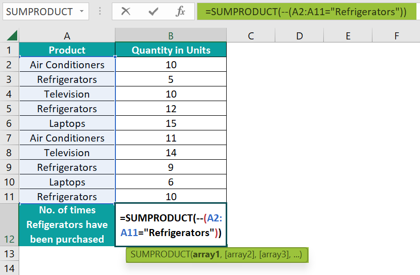
Step 2: Press Enter. You get the number of times “Refrigerators” occurs in the array A2:A11.

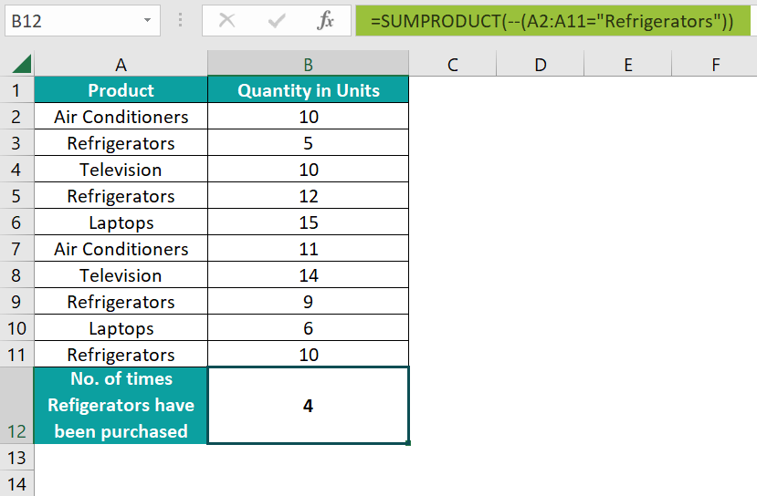
Thus, this is like using COUNTIF with SUMPRODUCT in Excel to count cells.

In the next part, we will see the other uses of the SUMPRODUCT function.

Example #2 – SUMPRODUCT Function with MOD

In this example, we must find the total revenue earned by a software firm from its different business units. Given below is a table containing the revenue information. Column A gives the name of the various departments, and Column B shows their respective revenues. We have used the SUM function in rows 5,9, and, and 13 to find the revenues of individual divisions.

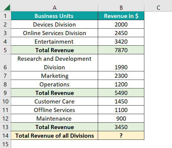
SUMPRODUCT Function in Excel - Example 2

Step 1: To get the total revenue, we must add the revenues of each unit in every fourth row(Rows 5,9,13). So, apply the following function in cell B14.

=SUMPRODUCT(B2:B13*(MOD(ROW(B2:B13)-1, 4)=0)).

Here, the innermost ROW excel function returns the row number of each row. For instance, =ROW(B3) returns 3.
However, we already have one row for headings. So, we subtract one (1) from the ROW function’s result to get the row number.
Now, use the MOD Excel function to check for those rows with zero remainders(rows 5,9, and 13).
MOD(ROW(B2:B13)-1, 4)=0 returns { FALSE, FALSE, FALSE, TRUE, FALSE, FALSE, FALSE, TRUE, FALSE, FALSE, FALSE, TRUE}. Every fourth row is returned as TRUE.
Now, SUMPRODUCT gets the total revenue in those rows, which returns TRUE.

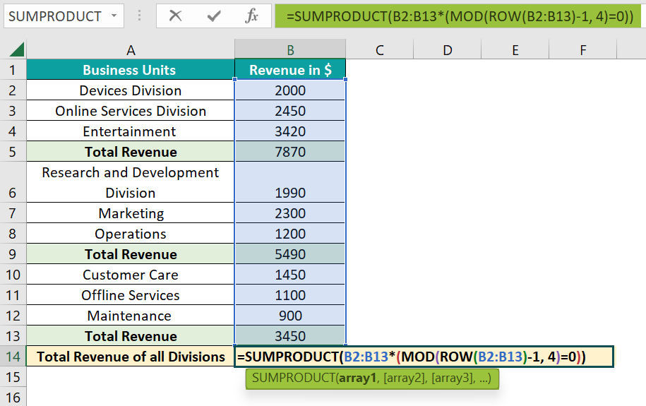
Step 2: Press Enter. Thus, cell B14 gives the total revenue earned by the businessman.

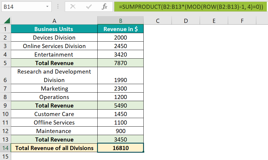
Here, the formula gives the result of $16,810. The SUMPRODUCT function can perform several complex calculations when used with other functions.

Example #3

We can use SUMPRODUCT in Excel to calculate the weighted average. For instance, five projects are given to a student, each with a different weight. The final grade depends on will depend on the weightage of each project and the final exam. Let us have three columns. Column A represents the various projects, Column B the marks secured, and Column C the weightage.

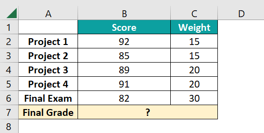
Step 1: Now, we use SUMPRODUCT to enter the two ranges, B2:B6 and C2:C6. Then, we divide it using the SUM on the weights.

Enter the formula: =SUMPRODUCT(B2:B6, C2:C6)/SUM(C2:C6) in B7.

SUMPRODUCT multiplies each score with the corresponding weight, then adds all these values together.
So, the projects with more weight are given a bigger weightage and have a bigger say in the final grade. So, the actual calculation of SUMPRODUCT(B2:B6, C2:C6) is as follows:

(92*15)+ (85*15)+ (89*20)+ (91*20)+ (82*30)

Now, the SUM excel function is used to bring the value down to the correct final score. The weights do not have to add up to 100% since we are dividing by the sum of the weights.

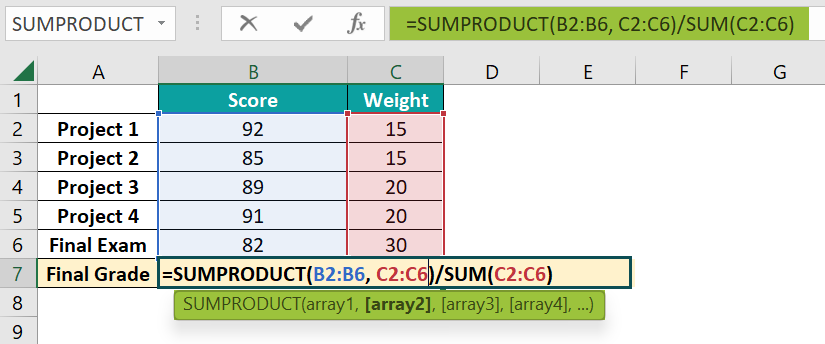
Step 2: Press Enter. You get the final score after weighing each project and exam score according to their value.

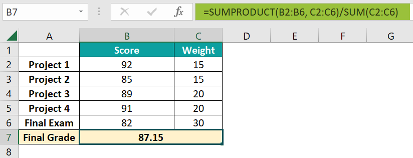
Thus, the weighted average can be easily calculated using the SUMPRODUCT function.

Important Things to Remember

In SUMPRODUCT, the array arguments should have similar dimensions; else, you get the #VALUE error. For instance, =SUMPRODUCT(A2:A6, B1:B3) gives an #VALUE error since the ranges aren’t the same size.
SUMPRODUCT can create array formulas without the complexity of using Ctrl + Shift + Enter.
SUMPRODUCT treats non-numeric array entries as zeros.
It can be used to count, add specific rows, and find the weighted average that otherwise involves complex formulas.

Frequently Asked Questions (FAQs)

1. How to add two SUMPRODUCT in Excel?

To add two SUMPRODUCT in Excel, all you need to do is to write the SUMPRODUCT function with the required criteria twice. For example, if you want to find the sum of the products of different numbers written in different columns, you can write the formula
=SUMPRODUCT(range) + SUMPRODUCT(another range).

2. How to round a SUMPRODUCT in Excel?

You can round the values first using the ROUND function in a separate column. Then, you can apply the SUMPRODUCT function to this column. Thus, the values are rounded off, and you can obtain the sumproduct.

3. Why is SUMPRODUCT in Excel not working?

If the different sets of arrays provided as arguments to the SUMPRODUCT function do not match in dimensions, you get the #VALUE! Error. Also, the function does not include non-numeric values and is treated as zeros.

4. What is the difference between sum and SUMPRODUCT in Excel?

The use of SUMPRODUCT in Excel is that multiplies the corresponding values in the arrays specified and returns their sum. SUM adds values in an array like in addition. You can add values, specific ranges, or cell references.

Download Template

This article must help understand SUMPRODUCT in Excel with its formula and examples. You can download the template here to use it instantly.

SUMPRODUCT in Excel Download

SUMPRODUCT in Excel