What Is Weighted Average In Excel?
The Weighted Average in Excel calculates the average of the numerical values, where the values contain assigned weighted percentage, from the overall percentage. The Weighted Average is calculated by finding the SUMPRODUCT of the values [multiply each value with its assigned weighted percentage] and the SUM of the weighted percentages and, finally, by dividing the SUMPRODUCT by the SUM.
Table of contents
Key Takeaways
- The Weighted Average in Excel helps the users find the mean of the numerical values containing the weight percentage.
- It is reliable because it gives more accurate results than the simple Average function.
- If the dataset contains text in the array range, the Weighted Average Formula considers the data value as 0.
- The Weighted Average in Excel function takes into account only the numerical values. So, when we assign a value for a text, then by the (–) double negative, Excel will convert “True” into 1 and “False” into 0. Then, we can proceed with the calculation.
Weighted Average Formula in Excel
The syntax of the Weighted Average formula in Excel is,
= SUMPRODUCT(array1,[array2],[array3],…) / SUM(number1,[number2],..)
How To Calculate Weighted Average In Excel?
We can Calculate Weighted Average in Excel in two ways,
- By manually selecting the excel cell reference with the values and multiplying it with its assigned weighted percentage.
- By using the Weighted Average formula in Excel.
Lets take a basic example where we Calculate Weighted Average in Excel without the use of formula.
In the table, the data is,
- Column A contains Values.
- Column B contains Weight.
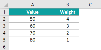
The steps to Calculate Weighted Average In Excel are as follows:
Step 1: Select cell B6 and enter the formula, =B2+B3+B4+B5. We get the output as “10” i.e., the weight total.

Step 2: Select the cell B7 and enter the formula, =(A2*B2+A3*B3+A4*B4+A5*B5)/B6
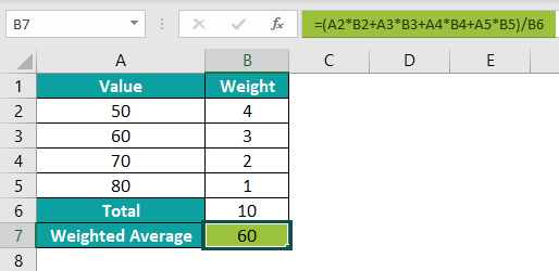
The output is shown above. The result of the Weighted Average is 60.
#1 – SUM Formula For Weighted Average
The SUM Excel function adds the values in a cell range and returns the sum.
The syntax of the SUM Formula for Weighted Average is,
=SUM(number1,[number2],..)
The arguments of the SUM Formula for Weighted Average are,
- number1 – We will add the first numeric value. It is a mandatory argument.
- number2 – We will add the second numeric value. It is an optional argument.
#2 – SUMPRODUCT Formula For Weighted Average
The SUMPRODUCT function multiplies the values in an array range and returns the sum of those products.
The syntax of the SUMPRODUCT formula for Weighted Average is,
=SUMPRODUCT(array1,[array2],[array3],…)
The arguments of the SUMPRODUCT formula for Weighted Average are,
- array1 – We will find the product of the first numeric range or array values and add them. It is a mandatory argument.
- array2 – We will find the product of the second numeric range or array values and add them. It is a mandatory argument.
- array3 – We will find the product of the third numeric range or array values and add them. It is an optional argument.
Examples
We will understand the Weighted Average in Excel with some advanced scenarios.
Example #1 – Weighted Average using SUMPRODUCT and SUM formula
We will find the Weighted Average using SUMPRODUCT and SUM formula.
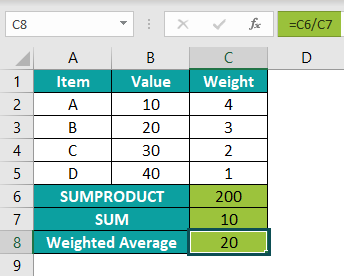
In the table, the data is,
- Column A contains Items.
- Column B contains Values.
- Column C contains Weight.

The steps to find the Weighted Average of the given values are as follows:
Step 1: First, select cell C6 to find the SUMPRODUCT.
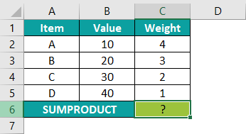
Step 2: In cell C6, enter the formula, =SUMPRODUCT(B2:B5,C2:C5) and press the “Enter” key.
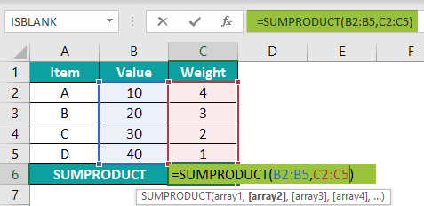
Step 3: The result of the SUMPRODUCT is ‘200’, as shown below.

Step 4: Next, select cell C7 to find the SUM.

Step 5: In cell C7, enter the formula, =SUM(C2:C5) and press the “Enter” key.

Step 6: The result of the SUM is ‘10’, as shown below.

Step 7: Now, select cell C8 to find the Weighted Average using SUMPRODUCT and SUM formula.

Step 8: In cell C8, enter the formula, =C6/C7 [ i.e., SUMPRODUCT / SUM], or select the cell references and press the “Enter” key.

Step 9: The output is ‘20’, as shown below.
Example #2 – Weighted Average With 0’s & 1’s Value Of SUMPRODUCT
We will find the Weighted Average with 0’s & 1’s value of the SUMPRODUCT formula.
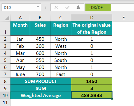
In the table, the data is,
- Column A contains Month.
- Column B contains Sales.
- Column C contains Region.
- Column D contains the original value of Region.
The tabular explanation of this example is as follows:
| Month | Sales | Region | The original value of the Region |
|---|---|---|---|
| Jan | 450 | North | True |
| Feb | 300 | West | False |
| Mar | 600 | North | True |
| Apr | 550 | South | False |
| May | 400 | North | True |
| June | 700 | East | False |
In the SUMPRODUCT function, we have assigned the formula to the text value “North”, and so the text assigned will have “True” or “False” values.
The function only uses the numerical values, so by the (–) double negative, Excel converts “True” into 1 and “False” into 0, as explained below.
[So, the value will return as 1 for “True” only for “North”]
| Sales | Region | SUMPRODUCT |
|---|---|---|
| 450 | 1 | 450 * 1 = 450 |
| 300 | 0 | 300 * 0 = 0 |
| 600 | 1 | 600 * 1 = 600 |
| 550 | 0 | 550 * 0 = 0 |
| 400 | 1 | 400 * 1 = 400 |
| 700 | 0 | 700 * 0 = 0 |
| Total of SUM = 3 | Total = 1450 | |
| Weighted Average | SUMPRODUCT / SUM | 1450 / 3 = 483.333 |
The steps to calculate the Weighted Average of the given values are as follows:

Step 1: First, in cell D8, enter the formula, =SUMPRODUCT(–(C2:C7=“North”),B2:B7)

Step 2: Press the “Enter” key. The result of the SUMPRODUCT is “1450”, as shown below.

Step 3: Next, in cell D9, enter the formula, =SUM(D2:D7)

Step 4: Press the “Enter” key. The result of the SUM is “3”, as shown below.

Step 5: Finally, in cell D10, enter the formula, =D8/D9 [i.e., the formula for calculating the Weighted Average in Excel, SUMPRODUCT / SUM].

Step 6: Press the “Enter” key. The Weighted Average result is “483.333”, as shown below.
Important Things To Note
- We can calculate the Weighted Average in Excel using the SUMPRODUCT and the SUM function or by selecting the cell references with the values and multiplying them with the assigned weighted percentage.
- Stock investors use the weighted average to track the cost of shares.
- The Weighted Average in Excel will return a “#VALUE!” error if the array arguments in the SUMPRODUCT function are of different sizes.

Frequently Asked Questions (FAQs)
The Weighted Average in Excel means providing the desired weights to each of the values available for calculating the average.
The Weighted Average formula in Excel is,
= SUMPRODUCT(array1,[array2],[array3],…) / SUM(number1,[number2],..)
A few ways to Calculate Weighted Average in Excel are as follows:
1) We can select the cell reference with the values and multiply it with its assigned weighted percentage.
2) We can use the Weighted Average formula [SUMPRODUCT and the SUM function]. We use the SUMPRODUCT formula to get the product of all the number range with available weights, find its sum, and then divide that with the actual SUM of the available weights.
3) We can use the AVERAGE function and multiply the numbers by their weightage.
Download Template
This article must help understand the Weighted Average in Excel with its formula and examples. You can download the template here to use it instantly.
Recommended Articles
This has been a guide to Weighted Average In Excel. Here we will calculate it manually & with the formula, along with examples & downloadable excel template. You can learn more from the following articles –

Leave a Reply