VLOOKUP With SUM

What Is VLOOKUP With SUM?

VLOOKUP function is useful whenever we want to retrieve values from a large data set based on certain values. It is often used to retrieve the scalar value or single value of the desired lookup value. However, VLOOKUP with SUM adds the sum of all the desired lookup values as an array function, to get the eventual result.

For instance, we have the following monthly product sales data in an Excel spreadsheet. In cell I2, we will find the total units sold for the product “Groceries”.

Select cell I2, enter the formula =SUM(VLOOKUP(H2,$A$2:$F$6,{2,3,4,5,6},0)), and press the keys “Ctrl + Shift + Enter”, as this is an array formula in Excel.

We get the output as 1559, for the lookup value of “Groceries”, as shown above.

What Is VLOOKUP With SUM?

In VLOOKUP with SUM, VLOOKUP will return multiple column values, and then the SUM function will add up those numbers to get the sum of multiple columns.
VLOOKUP can fetch the value from more than one column if we specify the column numbers in curly brackets.
VLOOKUP with SUM works without an array formula in the Office 365 version of Excel.
When we need to get the sum from multiple rows, VLOOKUP cannot fetch that. In such scenarios, we use the SUMPRODUCT function to match the criteria and get the sum from the matching rows.
Inside the SUMIF function, we can use the VLOOKUP function to get the criteria to value from a different table.

How To Use VLOOKUP With SUM?

Since Excel doesn’t have an inbuilt function for VLOOKUP With SUM, we can combine the VLOOKUP and the SUM Excel function.

The syntax of the combined VLOOKUP formula with the SUM formula is as follows,

=SUM(VLOOKUP(lookup_value,table_array,col_index_num,range_lookup))

lookup_value: The value for which we are trying to retrieve the result from the table array(2^ndargument). It is a mandatory argument.
table_array: This will be either a range or table array where we search for the lookup value. It is a mandatory argument.
col_index_num: From the given table_array, the columns we are looking for the result. Since we are retrieving the values from multiple columns, we need to mention all the required column numbers in a curly bracket ({}).
[range_lookup]: In this argument, we need to specify the kind of match we need to do:
- 0 or FALSE – It will search for the exact match of the lookup_value in the table_array. If nothing is specified, 1 or TRUE will be the default mode.
- 1 or TRUE – It will search for the approximate match of the lookup_value in the table_array.

Let us take a basic example to understand its usage.

We will find out the bonus for Feb of the employee “Sumit Bala” using VLOOKUP with SUM.

For instance, we have the following employee monthly bonus data in Excel.

How to Use VLOOKUP with SUM in Excel - Basic Example

The steps to find the required data using VLOOKUP with SUM are,

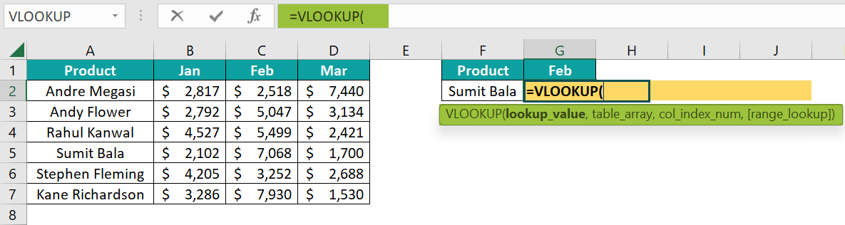
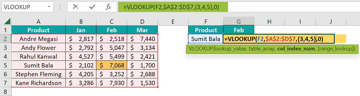
Select cell G2, and enter the formula =VLOOKUP(
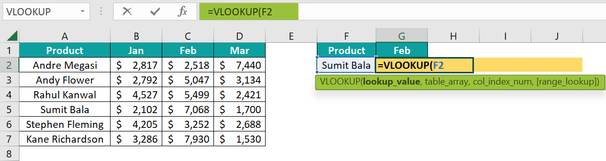
Choose the lookup_value as cell F2.
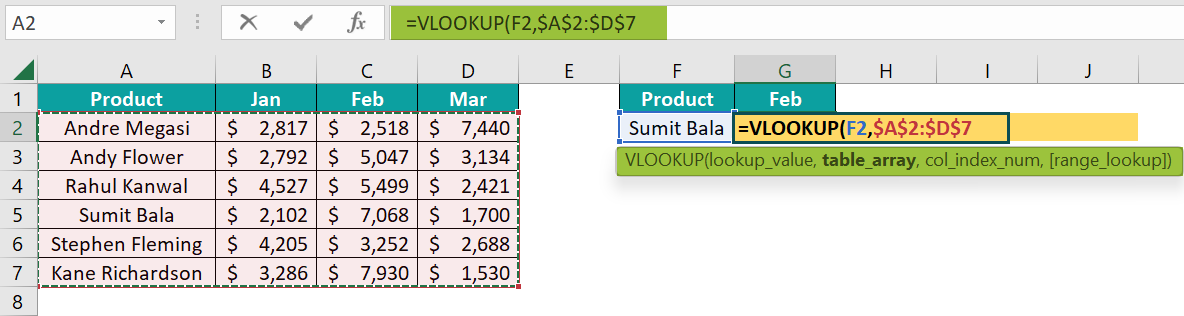
Choose the table array as A2:D7 and make it an absolute reference by pressing the F4 key.
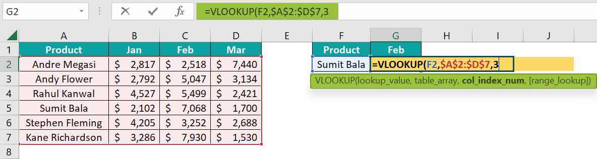
Next, enter the column number from which we need the result. Since we need the value from Feb month, enter the column number as 3.
Finally, mention the range lookup as an exact match by entering either FALSE or 0, then close the brackets, and press the “Enter” key. The complete formula so far is =VLOOKUP(F2,$A$2:$D$7,3,0)

The output, i.e., the bonus value of the employee “Sumit Bala” for the month of “Feb” is $7068, as shown above.

Now, instead of a single month, we need all the months total for the same employee, i.e., Jan, Feb, and Mar. For this, when entering the column number need to enter all the month’s column numbers in curly brackets ({}) as shown in the following image.

[Note: Column numbers {2,3,4} represent the column numbers for Jan, Feb, and Mar months.
However, if we hit the enter key, we get the #REF error value.]
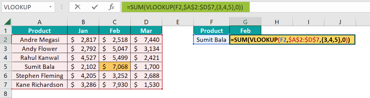
To get the correct result, we will now use the VLOOKUP with SUM formula.
Select cell G2, and enter the formula =SUM(VLOOKUP(F2,$A$2:$D$7,{3,4,5},0))
Press the “Enter” key, and we will get the #REF error, as shown below.

Since we have entered multiple column values, we must execute the formula as an array formula. So, press the keys “Ctrl+Shift+Enter”. Now the formula is =SUM(VLOOKUP(F2,$A$2:$D$7,{2,3,4},0))

The total bonus earned by the employee “Sumit Bala” in 3 months is $10,870.

Examples

We will understand some advanced scenarios using the VLOOKUP with SUM examples.

Example #1 – SUM of Matching Values in Columns

Now we will see how to get the sum of all the matching values from the column.

We have the following yearly units sold data of different products in Excel.

We have 6 years of units sold of products from A6:G16. Now we will find the total units sold for the products A, R, and C.

The steps to calculate the VLOOKUP with SUM are,

Step 1: Select cell B2, and enter the formula =VLOOKUP(

Step 2: Choose the lookup value as cell A2.

Step 3: Choose the table array from A7:G16 and make it an absolute reference in Excel by pressing the F4 key, so that when we copy the same table array reference to the below cells, it should be static.

Step 4: Next, we need to enter from which columns we need the data. Since we are looking for all the year’s data, enter the column numbers as {2,3,4,5,6,7}, in curly brackets ({}).

Step 5: At the last of the VLOOKUP, give the matching type as FALSE or 0 to get the exact match.

Step 6: Now wrap the VLOOKUP with SUM function. The complete formula is =SUM(VLOOKUP(A2,$A$7:$G$16,{2,3,4,5,6,7},0))

Step 7: If we are using the Office 365 version of Excel, then we can simply hit the “Enter” key to get the result. And, if we use any other versions, execute the formula with the Ctrl+Shift+Enter key.

VLOOKUP with SUM in Excel - Example 1 - Step 7a

The total number of units sold across years for product A is 2,40,434. Now, drag the formula from cells B2 to B4 using the excel fill handle.

We got the result as #N/A for product R in cell B3 because product R is not found in the sales table range A6:G16.

To tackle these errors, wrap the entire SUM and VLOOKUP formula with the IFERROR excel function as,

VLOOKUP with SUM in Excel - Example 1 - Step 7c

Whenever there is an error, the IFERROR will convert the error cell into a blank value, as shown above.

Example #2 – SUM of Matching Values in Rows

When the data contains multiple records of the same item, then we need to come up with a different strategy.

For instance, we have the following data in Excel. In the below data, we have multiple entries for products A & C. To get the sum from the multiple columns, we cannot use the VLOOKUP function; instead, we will use the SUMPRODUCT excel function.

The steps to calculate using the SUMPRODUCT function are,

Step 1: Select cell B2, and enter the formula =SUMPRODUCT(

Step 2: For the array1 argument, choose the product name list from D2:D10.

Step 3: Enter an equal sign and give the excel cell reference of the A2 cell.

Step 4: Surround this logic with brackets. Doing so will check all the rows in the range D2:D10 that are equal to the value in cell A2.

Step 5: Enter the multiple sign asterisk (*) and select the range from table E2:J10.

Step 6: Close the brackets, and press the “Enter” key to get the result. The complete formula is =SUMPRODUCT(($D$2:$D$10=A2)*$E$2:$J$10)

VLOOKUP with SUM in Excel - Example 2 - Step 6

Here, the SUMPRODUCT function looks for all the matching records of product A and summates all the matching rows. So, the total units sold for product A is 11,500, and C is 7,744.

Example #3 – VLOOKUP with SUM

We have the following employee table in Excel. We have 3 tables, A, B, and C.

In table A, we have a unique Product Name and ID, and in table B, we have product id-wise units sold data.

In table C, we need to get the sum of total units sold based on the product name.

Here, we do not have a product name in table B to find the sum of units sold from table B based on the product name. Therefore, we will combine SUMIF and VLOOKUP to arrive at the result here.

To calculate the VLOOKUP with SUM, first, select cell H3, and enter the formula =SUMIF(

Choose the range as the product id list from table B, D3:D10.

Now we must have the criteria to consider the product id, but we have the criteria as product name, and not product id. So, based on the product name, we will fetch the product id from table A by using the VLOOKUP function.

Using the VLOOKUP function, we retrieve the product id for product A from table A. Next, enter the sum range as the unit’s column from table B.

Close the bracket and press the “Enter” key to get the sum of all the rows of product A. The complete formula is =SUMIF($D$3:$D$10,”=”&VLOOKUP(G3,$A$3:$B$6,2,0),E3:E10)

VLOOKUP with SUM in Excel - Example 3 - Step 4

The total number of units for product A is 11,992.

Important Things To Note

When we supply multiple column numbers in the VLOOKUP function, we need to enter the column numbers inside the curly brackets ({}), each column number separated by a comma.
If we use the Office 365 version of Excel, we can press the “Enter” key to execute the formula as an array formula. However, if we are using Excel 2016 and earlier versions, then we need to execute the formula as an array formula using the Ctrl + Shift + Enter key.
The array formula will have the curly brackets on either side of the formula that is not visible in edit mode.
VLOOKUP can do the addition from only one row. If multiple rows exist for the same item, then we need to use the SUMPRODUCT function.

Frequently Asked Questions (FAQs)

1. Can I Use SUM and VLOOKUP Together?

Yes, we can use the SUM and VLOOKUP functions together to get the value from multiple columns.

2. How to SUM and match VLOOKUP in a row?

Let us consider the following data in Excel to SUM and match VLOOKUP in a row.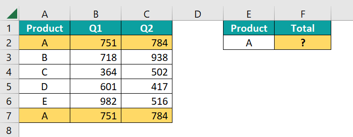

VLOOKUP with SUM - FAQ 2

We have multiple records for product A, select cell F2, and enter the formula =SUM(VLOOKUP(E2,$A$2:$C$7,{2,3},0))

FAQ 2 - Step 1

VLOOKUP retrieved the value from Q1 & Q2 for the first record of product A, i.e., row number 2.

However, it did not consider the second entry in the 7^th row for product A.

When we need to sum the values from multiple row values, we need to use the SUMPRODUCT function, as shown in the following image.

FAQ 2 - Step 2

SUMPRODUCT will find the records in the range A2:A7 for product A and then add the matching row values to get the values from multiple rows.

3. How to SUM and match a VLOOKUP column in Excel?

Let us look at the following data in Excel.

VLOOKUP with SUM - FAQ 3

For product C, we have three-quarters data. So, using the VLOOKUP with SUM, we will add multiple columns of data.

Select cell G2, and enter the formula =SUM(VLOOKUP(F2,$A$2:$D$6,{2,3,4},0))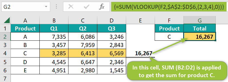

FAQ 3 - Step 1

VLOOKUP returns the values from the columns {2,3,4} and returns an array of values. Then SUM function will add those and returns the overall total as 16,267.
In cell E4, we have applied a simple SUM function to cross-check the result, matching with the VLOOKUP and SUM function results.

Download Template

This article must help understand the VLOOKUP With SUM with formulas and examples. You can download the template here to use it instantly.

VLOOKUP With SUM Download