
What Is SUMIF With VLOOKUP In Excel?
SUMIF function is used to get the sum of rows based on the criteria given and VLOOKUP is used to retrieve the value for the provided lookup value. SUMIF and VLOOKUP functions are an integral part of the Excel formulas family.
However, the combination of these two functions can solve various manual methods. Suppose the SUMIF criteria value is not available within the cell range where the SUMIF function is applied. We will use the VLOOKUP function to retrieve the value from the other table based on the common column between the two tables.
Use this SUMIF with VLOOKUP Template to follow along with the examples in this article.
Download Excel TemplateKey Takeaways
- SUMIF with VLOOKUP function helps us to find the matching value from different tables and return the criteria value for the SUMIF function
- SUMIF and VLOOKUP combination works well to match values in two tables and get the sum for the matching values.
- If no matching value is returned by the VLOOKUP function, the SUMIF function will return 0 as the total.
- The SUMIF and VLOOKUP functions can work to retrieve the values from the different worksheets as well as from different workbooks.
How Does Using SUMIF With VLOOKUP Help Users?
For instance, look at the following data in Excel.
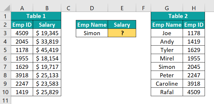
We have two tables Table 1 and Table 2.
In Table 1, we have Emp ID and their salary details and in Table 2, we have Emp ID and Emp Name.
In cell E2, we are trying to fetch the salary information based on the emp name from Table 1. However, in table 1 we do not have the emp name, so SUMIF cannot find the matching criteria value in the table for the emp Simon.
In these cases, we need to retrieve the emp ID for the emp name by using the VLOOKUP function to assist the SUMIF excel function.
The following image shows the combination of SUMIF and VLOOKUP functions to get the desired value.
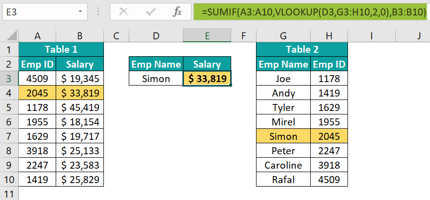
The salary sum for the emp name Simon is $33,819. Here, the VLOOKUP function retrieved the emp ID from table 2 based on the emp ID, then the SUMIF function will match the emp ID in table 1 and return the sum of salary for the desired employee.
How To Use SUMIF With VLOOKUP In Excel?
When we deal with the SUMIF function, we need to understand the syntax first. The following image shows the syntax of the SUMIF function in Excel.
- Range: The range of cells where we need to evaluate the criteria.
- Criteria: In the provided range what cells do we need to use for sum values.
- [Sum Range]: The range of cells that we need to sum in the given range and criteria.
The syntax of the VLOOKUP function is

- Lookup_value: The value for which we are trying to retrieve the result from the table array (2rd argument). It is a mandatory argument.
- Table_array: This will be either range or table array where we search for the lookup value. It is also a mandatory argument.
- Col_index_num: From the given table array from which column, we are looking for the result.
- [Range_lookup]: In this argument, we need to specify the kind of match we need to do:
- 0 or FALSE – This will search for the exact match of the lookup value in the table array. If nothing is specified 1 or TRUE will be the default mode.
- 1 or TRUE – This will search for the approximate match of the lookup value in the table array.
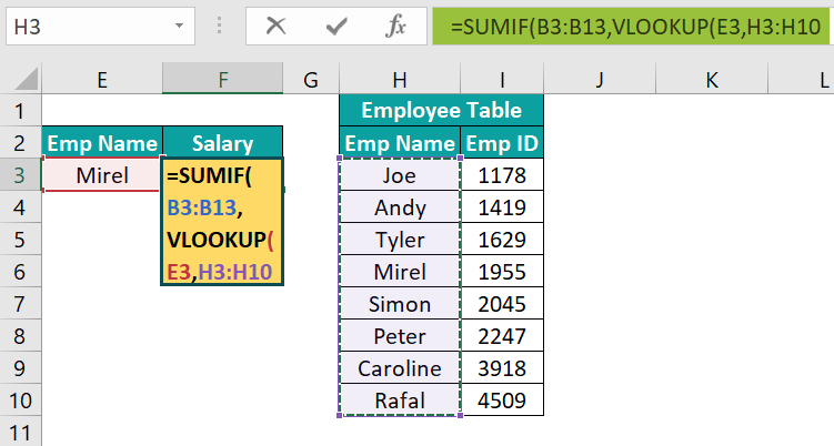
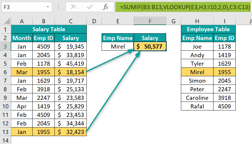
Now, let us apply these two functions to get the functionality together. We have the following two table data in Excel.
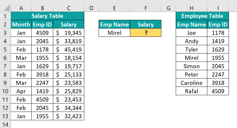
We have two tables Salary Table and Employee Table.
In Salary Table, we have monthly payout data with employee ID, but we do not have employee name in this table.
In Employee Table, we have Employee Name and Employee ID.
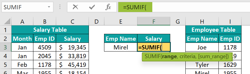
Now, in cell F2, we need to get the total salary paid for the employee MIREL across months by using the employee’s name from the Salary Table.
However, the issue here is we do not have the employee’s name in the Salary Table. To solve this issue, we will use the combination formula of SUMIF and VLOOKUP.
- First, enter the SUMIF function in cell F2.

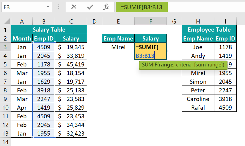
- Then, choose the range from B2:B13 from the Salary Table.

- Next, for the criteria, we need to give which employee ID to be considered. However, as a criteria, we have the employee name instead of the employee ID in cell E2.
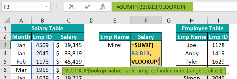
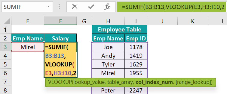
To get the employee ID from the Employee Table, we will use the VLOOKUP function. Hence, enter the VLOOKUP function within the SUMIF function.

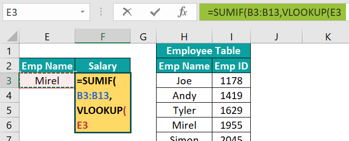
- Now, enter the lookup value as the employee name in cell E2.

- Next, enter the table array from H2:I13 in the Employee Table.

- Then, enter the column index number as 2 to get the employee ID from the second column of the table array selection.

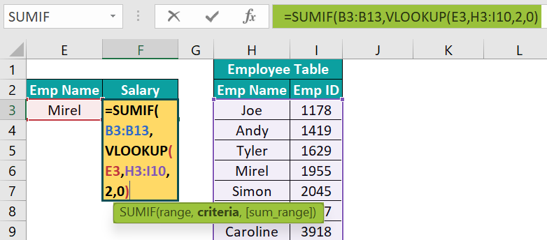
- Next, enter the matching criteria as FALSE to get the exact match.

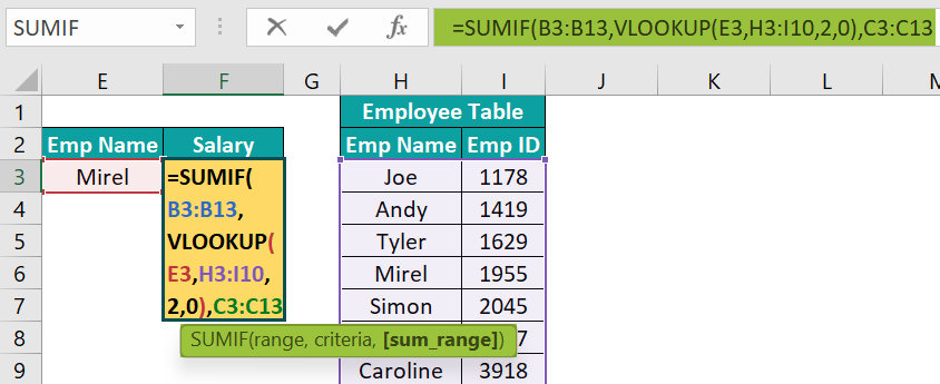
Here, what the VLOOKUP function does is, it will fetch the employee ID for the employee’s name in cell E2 and then SUMIF will match the same employee ID if range B3:B13. - Now, we need to give the sum range for the SUMIF function from C3:C13 once the VLOOKUP function is applied.

Next, close the bracket and then, hit the Enter key to get the result.
We have the total salary paid for the employee Mirel, even though we do not have the employee’s name in the Salary Table.
Therefore, using VLOOKUP function, we can retrieve the employee ID from the Employee Table.
Examples
Example #1 – Use Of SUMIF And VLOOKUP Together To Determine Some Value
To get the sum of certain when the value is appearing multiple times, we will use the SUMIF function, However, in some cases, we may not have the criteria value readily available in the main table; rather it will be in a different table.
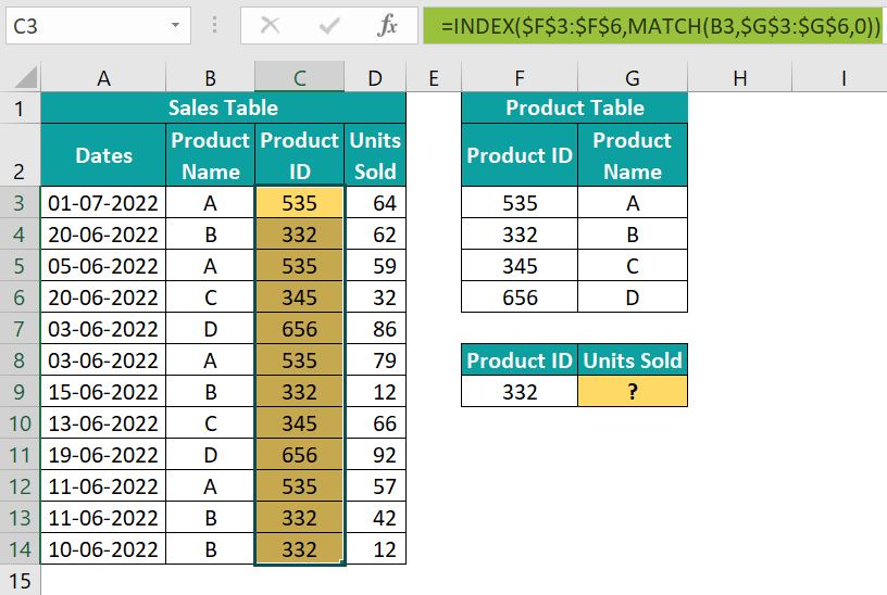
For instance, we have the following sales table and product table in an Excel spreadsheet.

In the sales table, we have products sold on different dates and each product is appearing multiple times in this table. In this table, we have only the product name and units sold on different dates.
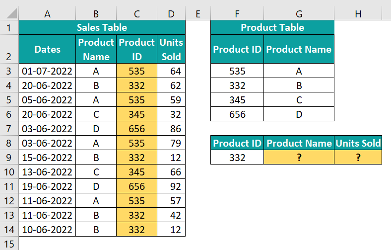
In cell F9, we need to find the total units for the product ID 332. However, we do not have the product ID in the Sales Table where SUMIF will be applied to get the total units sold for the product.
However, in the Product Table, we have the product name for each product ID. Now, we can insert a new column to get the product ID in the Sales Table like the following one.
Now, we have used the INDEX excel function and MATCH excel function to get the product ID from the Product Table. Since we have the product ID column now, we can apply the SUMIF function to get the sum of units sold based on product ID.
However, this isn’t the ideal way of getting things done because unnecessarily we have added a new column. Now let us find a way to eliminate this unnecessary column.
Method #1 – Find Product Name For The Product ID
One way to do it is by finding the product name for the given product ID. Now, let us understand this method with the following example.
First, enter the VLOOKUP function in cell G9.
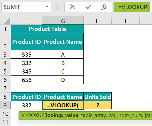
Next, choose the lookup value as a cell F9.
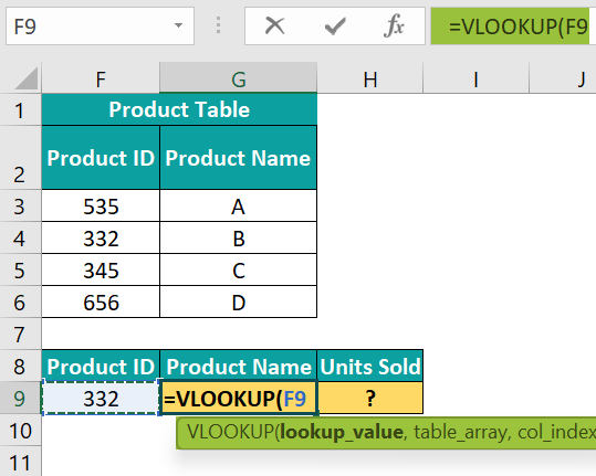
Then, choose the table from F3:G6 in the Product Table.
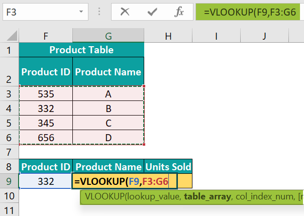
Now, enter the column index number as 2.

Next, enter the matching type as FALSE or 0 to get the exact match.
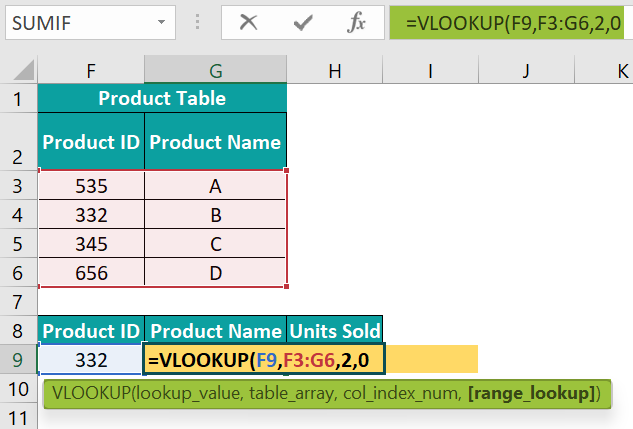
Then, close the bracket and hit the Enter key to get the product name.
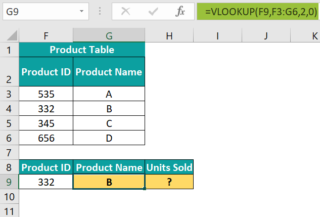
Now, in cell H9, apply the SUMIF function to get the total units sold for product B.
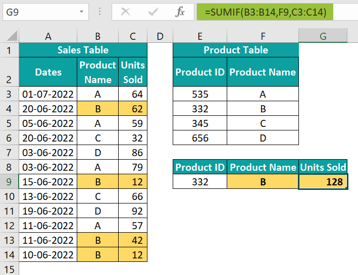
Clearly, we can see that all the colored cells in the Sales Table (cells C4, C9, C13, and C14) are summed up in cell G9 using the SUMIF function.
This looks much better than the previous one of adding a new column in the Sales Table. However, finding the product name and then entering the SUMIF function aren’t the best practices.
Instead of adding a new cell to find the product name, we can combine the VLOOKUP function with the SUMIF function to get the summation in single cells itself.

In the criteria argument of the SUMIF function, we have used the VLOOKUP function. Here, the VLOOKUP function is retrieving the product name for the product ID in cell E9, and the SUMIF function will match that product name in the range B3:B14 and return the sum of the cells in the range C3:C14 for all the matching products.
Example #2 – Determining SUM Based On The Matching Criteria In Different Worksheets
When the criteria column for SUMIF is not available in the same table, we have used the VLOOKUP function to match values and then get the sum of the total.
For instance, look at the below scenario.
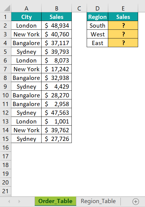
Now, in the Order Table worksheet, we have city wise orders.

Similarly, in the Region Table worksheet, we have the region and city which belongs to these regions.
Now, we need to find the sales for each region in the Order Table worksheet.

Next, apply SUMIF and VLOOKUP functions to get the sales value as we have applied in the previous example.

Here, the VLOOKUP function retrieves the city names for each region from another worksheet Region Table. Then, the SUMIF function matches those city names in the order table worksheet and returns the total sales for each region.
However, the SUMIF returns total sales only for the matching records. For instance, the region West SUMIF has not returned any value because in the Region Table worksheet, region West is not there.

VLOOKUP has not found any WEST region. So, it has not returned any of the matching cities for the SUMIF and SUMIF returned zero as the total sales for this region.
As soon as the WEST region is added to the Region Table, we will get the matching city value and SUMIF will return the total sales for that region.
Important Things To Note
- The SUMIF function matches only one criterion. Hence, if you want to match multiple criteria, then you need to use the SUMIFS function.
- The SUMIF sums the values only for the matching values returned by the VLOOKUP function.
- SUMIF and VLOOKUP combination can be applied to sum numerical values only.
- Always avoid adding a helper column first to retrieve the criteria column to assist the SUMIF function. This will just increase the memory of the Excel file.
Frequently Asked Questions (FAQs)
When we have the criteria value in a different table, we need to create a helper column first to retrieve the criteria column to assist the SUMIF function.
However, with the help of the VLOOKUP function, we can use this as an assisting function for the SUMIF function, and without creating a helper column we can still get the total sum.
For instance, look at the following two tables in Excel.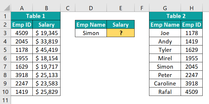
In Table 1, we do not have the employee’s name, but we need to sum the values based on the employee’s name. In Table 2, we have the employee ID based on the employee’s name.
So, the VLOOKUP function can be used here to retrieve the employee ID for the desired employee name, and then the SUMIF function will sum the values for the matching records in Table 1.
If we are facing the problem of SUMIF with VLOOKUP not working, then one possible reason would be to look at the lookup value in both tables. Also, the VLOOKUP function looks for the exact match in both the tables, so even if small spacing will results in a not available error and the SUMIF function end up returning no value for that lookup value.
To use VLOOKUP in the SUMIF function, the table should be designed in such a way that all the resulting columns should be to the right of the lookup value column and the data structure should be vertical only.
If our resulting column is to the left of the lookup value column, then VLOOKUP does not work.
Use this SUMIF with VLOOKUP Template to follow along with the examples in this article.
Download Excel Template