
What Is SUMPRODUCT With Multiple Criteria In Excel?
The SUMPRODUCT with multiple criteria in Excel compares data in multiple arrays and calculates the output based on more than one criterion. And the formula uses a double unary operator (‘– –‘) for each criterion or multiplies the criteria with 1 to convert TRUEs and FALSEs into 1s and 0s, respectively.
Users can use the SUMPRODUCT() with multiple criteria to apply sum product logic in a bond’s data with numerous conditions.
Use this SUMPRODUCT With Multiple Criteria Template to follow along with the examples in this article.
Download Excel TemplateFor example, the first table contains items, their grade, price, and order details.

Suppose the requirement is to calculate the total price of Grade B Maize. Also, if we have to display the result in cell C12, which has the data format set as Currency. Then, using SUMPRODUCT with multiple criteria in the target cell will fetch us the required data.

In the above example, the SUMPRODUCT() includes two criteria. It checks for the item Maize in the range A2:A9 and Grade B in cell range B2:B9.
And as the criteria hold in rows 4 and 8, the SUMPRODUCT() multiplies the rows 4 and 8 values in the specified columns C and D cell ranges. In other words, the function multiplies cells C4 and D4 values and cells C8 and D8 data. And then, it adds the products to return the total price of Grade B Maize as $63,910.00.
Key Takeaways
- The formula for SUMPRODUCT with multiple criteria evaluates the specified conditions and calculates the output with the qualifying array values.
- Users can use the SUMPRODUCT function with multiple conditions in scenarios, such as when determining the sum product in financial statistics with multiple criteria.
- The SUMPRODUCT() accepts the criteria with double unary operator and array values to manipulate as the arguments. Otherwise, the function accepts the products of all criteria and one or the array values to manipulate as the argument.
- Using SUMPRODUCT function containing multiple conditions, with inbuilt functions such as IF, DATE, LEN, and VLOOKUP, gives practical solutions.
SUMPRODUCT With Multiple Criteria() Excel Formula
The SUMPRODUCT() syntax is:

where,
- array1: The first array whose values we must multiply and later add. And it is a mandatory argument.
- array2, array3, …: The optional 2 to 255 array arguments whose values we require to multiply and later add.
But the SUMPRODUCT with multiple criteria formula is:

Or

In the first formula, arrays are the cell ranges separated by commas, whose values we require to multiply and later add. And in the second formula, arrays are all the cell ranges to multiply with the specified criteria and whose values we require to multiply and later add.
How To Use SUMPRODUCT With Multiple Criteria Excel Function?
We can use the SUMPRODUCT with multiple criteria Excel function in two ways, namely:
- Access from the Excel ribbon.
- Enter in the worksheet manually.
Method #1 – Access From The Excel Ribbon
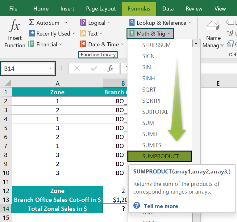
Choose the target cell for output.
Next, select the Formulas tab.
Click the Math & Trig option drop-down → select the SUMPRODUCT function, as shown below.

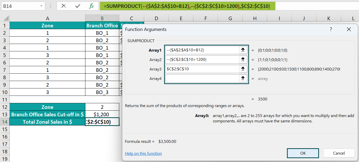
The Function Arguments window opens. Enter the arguments as the required criteria and arrays in the specified fields → click OK, as depicted below.
Though Excel shows three fields, the fourth field will appear once we click the third field. And we can enter up to 256 arguments in the SUMPRODUCT excel function.

Method #2 – Enter In The Worksheet Manually
- Choose the target cell for the output.
- Type =SUMPRODUCT( in the cell. [Alternatively, type =S or =SUM and double-click the SUMPRODUCT function from the Excel suggestions.]
- Enter the arguments as cell values or references and close the brackets.
- Press Enter to execute and view the outcome.
Let us take an example to learn more about this –
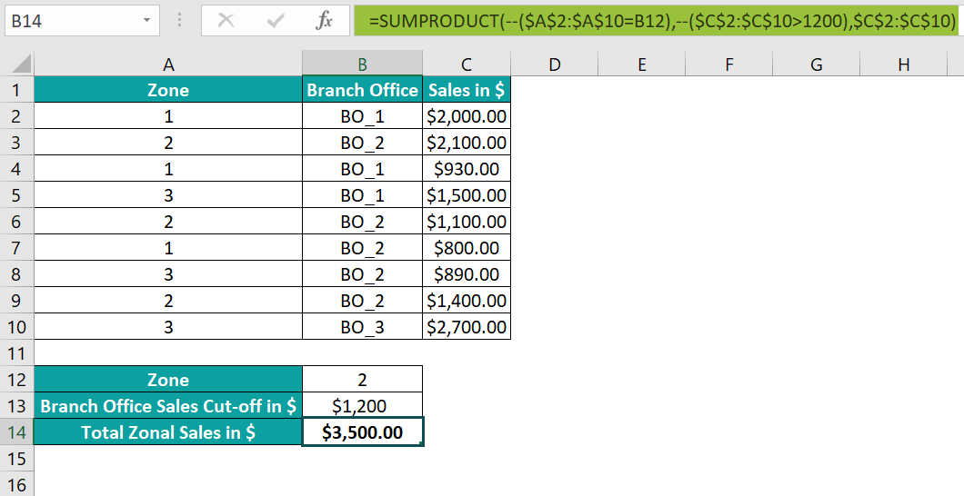
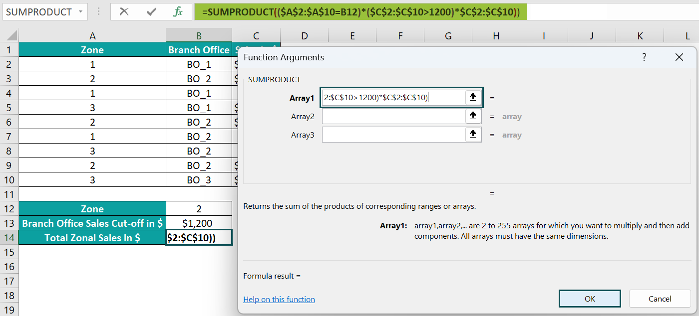
The below table shows the sales figures of branch offices in various zones.

Suppose the requirement is to determine the total sales in Zone 2. But the condition is that we must consider only those cells where the sales figure of a Zone 2 branch office is greater than $1,200. And assume the target cell is B14, which has the Currency data format.
Steps to use Sumproduct excel function with mulitple criteria are as follows –
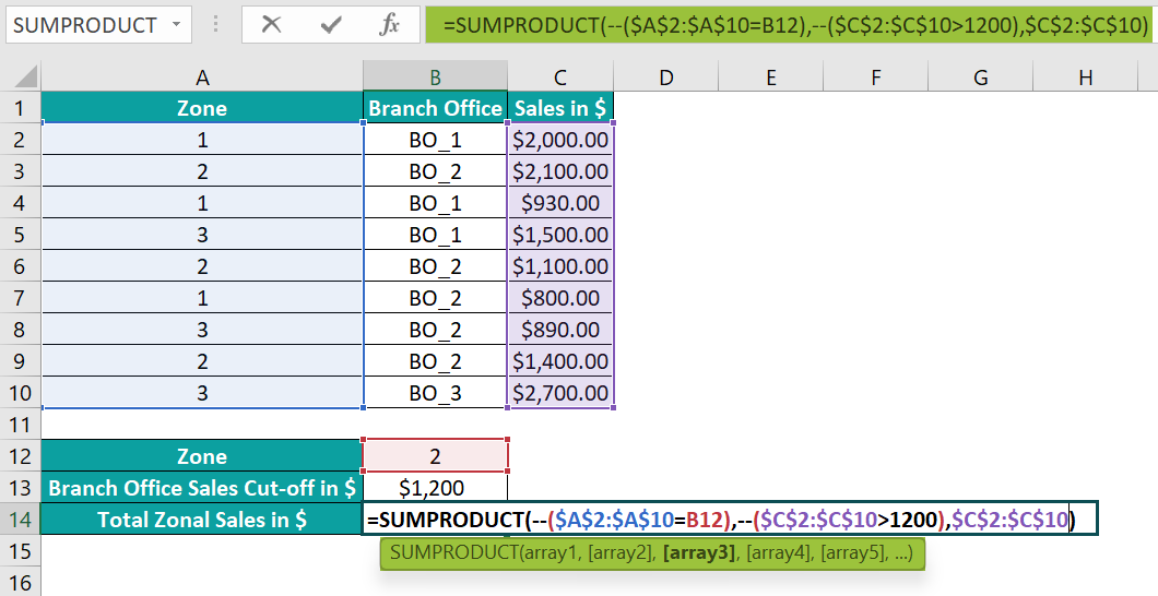
- Select the target cell B14 and enter the following SUMPRODUCT().
=SUMPRODUCT(–($A$2:$A$10=B12),–($C$2:$C$10>1200),$C$2:$C$10)

- Press Enter to view the required total sales in Zone 2.
On the other hand, the below formula will also give the same result.
=SUMPRODUCT(($A$2:$A$10=B12)*($C$2:$C$10>1200)*$C$2:$C$10)
[Alternatively, select the target cell B14, and navigate the path Formulas → Math & Trig → SUMPRODUCT to apply the SUMPRODUCT function in the chosen cell.
The above step will open the Function Arguments window.
Next, enter the given cell range references for the criteria and values to manipulate in the respective fields in the Function Arguments window.
Otherwise, we can update the Array1 field, as shown below, to get the required data.
Finally, click OK. The window will close, and we will obtain the SUMPRODUCT() output in the target cell B14.
The above example explains the two SUMPRODUCT with multiple criteria formulas.
The function in the two formulas checks two criteria to determine the cells in column A containing the Zone as 2 and the cells in column C where the sales figure exceeds $1,200.
The criteria return results as arrays of TRUEs and FALSEs. But the double unary operator in the first formula, ‘– –‘, converts the results into arrays of 1s and 0s.
For instance, the first criterion in the above function returns {FALSE;TRUE;FALSE;FALSE;TRUE;FALSE;FALSE;TRUE;FALSE}. The TRUEs indicate cells containing Zone 2. And the double unary operator changes the above array range as {0;1;0;0;1;0;0;1;0}.
Likewise, the double unary operator makes the second criteria output as {1;1;0;1;0;0;0;1;1}, with the 1s indicating cells containing sales values greater than $1,200.
And as the second and eighth elements in the two arrays are 1, the cells C3 and C9 values get added to give the result as $3,500.
In the case of the second formula, the criteria outputs are array ranges of TRUEs and FALSEs, as explained above. But the function multiplies the two array ranges with the specified array range of values we require to manipulate. And hence, the cells C3 and C9 values get added for the same reason mentioned previously.

Examples
Check out the following examples of SUMPRODUCT with multiple conditions to use the formula effectively.
Example #1
The table below contains the details of the country-wise votes for a set of branded products.

And we need to determine the total votes secured by the Apple brand in the UK and display the output in cell I3.
The above-mentioned requirement is a case of SUMPRODUCT with multiple criteria rows and columns. So, here is how to use the SUMPRODUCT() in the target cell and obtain the required vote data.
- Step 1: Select the target cell I3, enter the below formula, and press Enter.
=SUMPRODUCT((C2:F2=I1)*(B3:B11=I2)*C3:F11)

The above formula for SUMPRODUCT with multiple criteria rows and columns checks two criteria. It looks for cells containing the country name UK in the cell range C2:F2 (row 2) and the Apple brand in the cell range B3:B11 (column B). And the two criteria outputs are {FALSE,FALSE,TRUE,FALSE} and {TRUE;TRUE;FALSE;FALSE;TRUE;FALSE;FALSE;TRUE;FALSE}.
Finally, the formula multiplies the values in the range C3:F11 to the above-mentioned arrays. And it adds column E cell values in the rows where the corresponding column B cells contain the Apple brand, 1900, 4200, 1800, and 2500 (cells E3:E4, E7, and E10). These cells qualify because the third element is TRUE (column E) in the first criteria output. And the first, second, fifth, and eighth elements in the second argument are TRUE (rows 3, 4, 7, and 10). So, the intersection points of these elements are cells in the range E3:E4, E7, and E10. And thus, the total customer votes for Apple in the UK become 10400.
Example #2
The below table contains a list of fruits and their order details.

Suppose we need to assess the total number of boxes of Peach ordered between 15th January and 1st March 2022 and display the total in cell F3.
Then, we can use the formula for SUMPRODUCT with multiple criteria and date range as one of the conditions in the target cell to achieve the required data.
- Step 1: Select the target cell F3, enter the below formula, and press Enter.
=SUMPRODUCT(–($A$2:$A$11=F1),–(DATE(2022,1,15)<=$B$2:$B$11),–($B$2:$B$11<DATE(2022,3,1)),C2:C11)

The above formula for SUMPRODUCT with multiple criteria and date range contains three criteria.
The first condition checks for cells in the range A2:A11, which contain the fruit, Peach. The second and third conditions check for cells where the specified date range criteria hold. And in these two conditions, we use the DATE excel function to ensure the entered date values are valid.
So, the three criteria return arrays of TRUEs and FALSEs, and the double unary operator changes the array values to 1s and 0s, as explained in the previous sections. And as the conditions hold in rows 7 and 8, the function adds the cells in the range C7:C8 values to return the total number of boxes of peaches in the specified date range as 470.
Example #3
The first table shows the accounts in a firm and the bonus encashment details of employees in these accounts in different designations.

Suppose the requirement is to determine the total bonus encashment for headcounts in the given account holding the specified designation and display the outcome in cell G3. Assume the cell G3 format is Currency.
Then, we can apply the formula for SUMPRODUCT with IF multiple criteria as an array formula in the target cell and achieve the required output.
- Step 1: Select the target cell G3 and enter the below formula.
=SUMPRODUCT(IF(A2:A11=G1,1,0),IF(B2:B11=G2,1,0),C2:C11,D2:D11)

- Step 2: Press Ctrl + Shift + Enter keys to execute the above expression as an array formula.
{=SUMPRODUCT(IF(A2:A11=G1,1,0),IF(B2:B11=G2,1,0),C2:C11,D2:D11)}

As the IF() checks cell ranges, we must apply the above SUMPRODUCT() as an array formula.
The above formula for SUMPRODUCT with IF multiple criteria checks two criteria, the IF functions.
The first IF() checks for cells with account as BDJ in the range A2:A11 and returns an array of 1s and 0s, where the 1s indicates the cells where the IF condition holds. The second IF() checks for cells with employee designation as Software Engineer in the range B2:B11. And it returns an array of 1s and 0s, with the 1s indicating the cells where the IF condition holds.
So, the two IF() outputs are {1;0;0;1;0;0;0;1;0;0} and {1;0;1;1;0;0;0;0;1;0}. And as the criteria hold in rows 2 and 5, the function multiplies the rows 2 and 5 values in columns C and D.
In other words, the function finds the product of cells C2 and D2 values, $1,000, and the product of cells C5 and D5 values, $1,600.
Finally, it adds the two products to return the required total bonus encashment for the software engineers in the BDJ account, $2,600.
Important Things To Note
- Ensure the formula for SUMPRODUCT with multiple criteria includes a double unary operator for each condition or multiplies the criteria with 1. Otherwise, the formula will throw an error.
- The SUMPRODUCT function with multiple criteria returns the #VALUE! error if the specified arrays you aim to manipulate have different dimensions.
- The SUMPRODUCT function with multiple conditions counts non-numeric values in the specified arrays as 0.
Frequently Asked Questions (FAQs)
The SUMPRODUCT with multiple conditions does not return text.
The reason is that the SUMPRODUCT function is not a Text function. And if it tries to process array values, which are text, such as finding the product of strings and numbers, the function will throw an error.
We can apply the OR logic in the formula of SUMPRODUCT with multiple conditions using the ‘+’ symbol between the specified criteria.
For example, the following table contains a list of items and their quantity and price details.
Suppose the requirement is to determine the total price when the item is Item_2 or Item_3 and display the output in cell B16, which has the Currency format.
Then, here is how we can apply the OR logic in the formula of SUMPRODUCT with multiple conditions in the target cell and achieve the required output.
• Step 1: Select the target cell B16, enter the below formula, and press Enter.
=SUMPRODUCT((A2:A11=B13)+(A2:A11=B15),B2:B11,C2:C11)
The SUMPRODUCT() checks two criteria.
The two conditions look for cells in the range A2:A11 that contain Item_2 and Item_3, respectively. And each criterion returns an array of TRUEs and FALSEs, with the TRUEs indicating cells containing the specified item.
Next, the formula adds the two resulting array ranges of TRUEs and FALSEs and returns an array {0;1;1;1;1;0;1;0;1;0}. Finally, it multiplies the columns B and C values in rows where the corresponding element in the above array is 1, that is, in rows 3 to 6, 8, and 10. And then, the formula adds the products to return the required total price when the item is Item_2 or Item_3 as $17,625.
The SUMPRODUCT with multiple conditions is not working, perhaps due to the following reasons:
• The supplied ranges of the arrays we require to manipulate based on the given criteria are not of the same dimensions.
• All the values in the arrays we require to manipulate based on the given criteria are non-numeric.
• We did not specify the double unary operator for each criterion.
• We did not multiply the criteria with one or the arrays you aimed to manipulate based on the specified criteria.
Use this SUMPRODUCT With Multiple Criteria Template to follow along with the examples in this article.
Download Excel Template