INDEX MATCH Multiple Criteria

What Is INDEX MATCH With Multiple Criteria

The INDEX MATCH function combination is an alternative to the VLOOKUP function. The INDEX MATCH With Multiple Criteria helps users to retrieve the required data in a dataset where we may not find a unique column to apply the lookup function. Therefore, in such scenarios, we find a pattern to identify the unique lookup_value column, and the multiple criteria columns to create a unique column to apply the lookup logic to retrieve values.

How To Use INDEX MATCH With Multiple Criteria?

First, we will understand what is meant by multiple criteria in the lookup function.

Consider the following data in Excel. We have product sales with different box types.

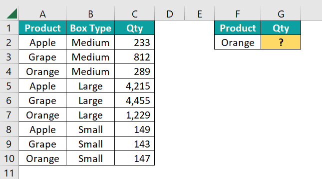
Step 1: First, let us apply the INDEX MATCH function, to retrieve the sales figure for the product “Orange”.

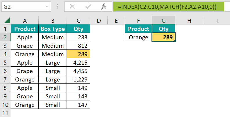
We have got the result as 289. But, let us look at the data closely to find the real problem.

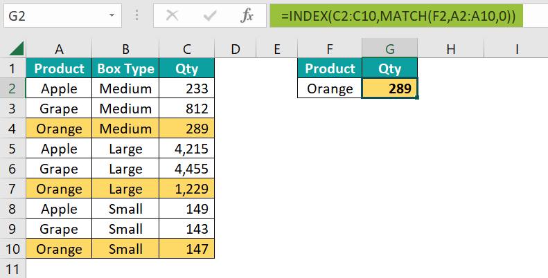
We have the product “Orange” appearing 3 times with different box sizes. That means the product is not a unique column to retrieve the value. INDEX MATCH function retrieved the value from the first matching record, and the first matching record quantity is 289.

When we try to retrieve the quantity value for the product, we must be sure which box type we are looking for. The “Product” is not the only criteria to retrieve the value, we must include the “Box Type” as the second criteria to find the quantity number for the specific box type and product.

Step 2: Let us modify the result table as follows.

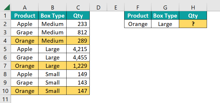
There is another problem here, i.e., we do not have the unique column yet, to apply the INDEX MATCH multiple criteria.

Step 3: First, we must create a unique column in the combination of “Product” and “Box Type”. Insert a new column called “Helper”, and apply the concatenation formula to combine the “Product” and “Box Type” columns with the pipe symbol “|” as the delimiter between these columns.

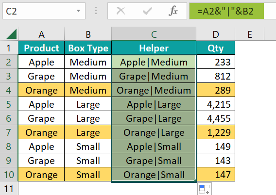
Now that we have the unique column in place, let us apply the INDEX and MATCH functions to retrieve the quantity for the specific product and box type.

Step 4: Enter the INDEX function in cell I2.

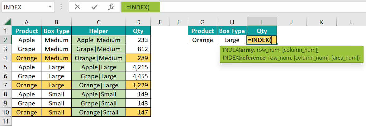
Step 5: Choose the array as the result column, i.e., the Quantity column from D2:D10.

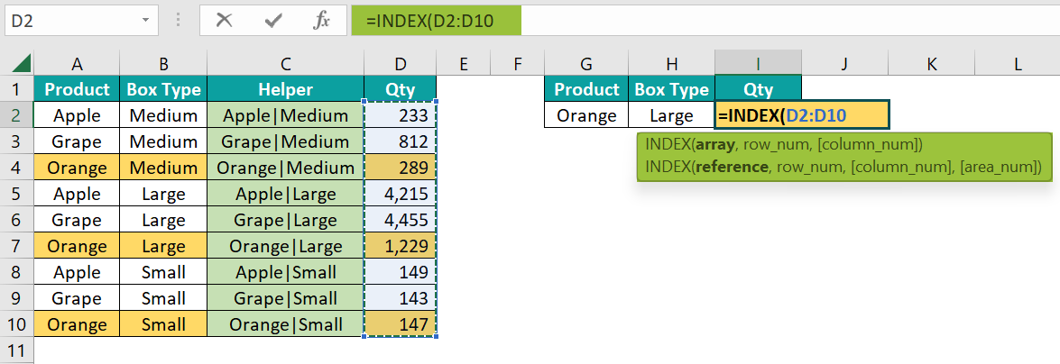
Step 6: Next, we must find the row number for the combination of the product “Orange” and box type “Large”. To find it dynamically, we will use the MATCH function in the row number argument of the INDEX excel function.

Now, we must choose the lookup_value for which we must find the row number. However, we do not have a single lookup_value here, but we have two.

Step 7: We have created a unique column in the table by combining the Product and Box Type. Let’s combine these two columns in the lookup_value in the same manner we have created the lookup_value column.

Step 8: Choose the lookup array from C2:C10.

Step 9: Enter the matching type as 0 to get the exact match.

Step 10: Close the brackets of both the INDEX and MATCH functions and hit the enter key to get the result.

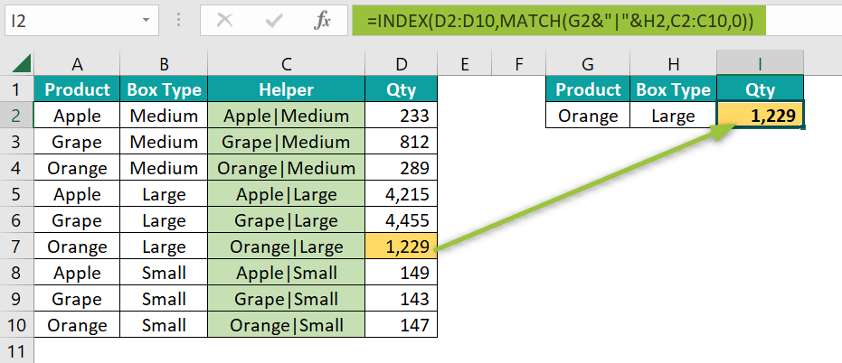
Now the INDEX and MATCH formula retrieves the correct value. We can change the Product Name in cell G2, and Box Type in cell H2, to get the corresponding quantity value.

For instance, look at the following image.

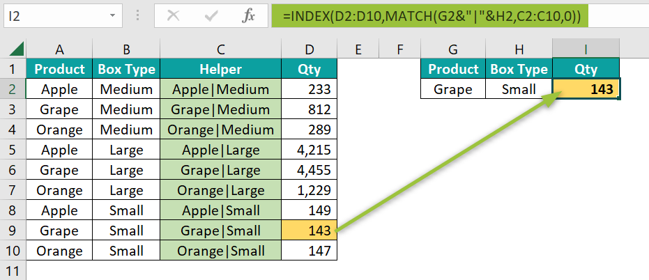
The formula returns the quantity value for the product “Grape”, and box type “Small”.

Advanced Examples

We will consider some advanced examples of INDEX MATCH multiple criteria, namely,

1. Two INDEX functions and a MATCH function with Multiple Criteria.
2. Using INDEX with Two MATCH functions with Multiple Criteria in Excel.

Example #1

• Two INDEX functions and a MATCH function with Multiple Criteria

In the above example, we have used the helper column to get the quantity value. Now, let us understand retrieving the values without the helper column.

We are using the same data from the previous example. Here, the challenge is to find the row number for multiple criteria like product and box type.

First, let us understand how to find the row number for the given product and box type.

Enter the MATCH function in cell H2.

Choose the lookup_value as cells F2 and G2 with the ampersand symbol to concatenate together.

This combination shows that we are trying to find the row number for these two matching records in the table.

Next, to choose the lookup array, we do not have the helper column. Hence, enter the INDEX function to choose the lookup array.

First, choose the product array from A2:A10.

Then enter the ampersand (&) symbol and choose the box type array from B2:B10.

Enter a comma (,), and close the bracket of the INDEX function.

For the MATCH functions, the last argument enters 0 to get the exact match.

Close the bracket and press the “Enter” key to get the row number for the given combination of product and box type.

It returns the row number of the position of the given combination of the product and box type, i.e., 8.

We can combine this with another INDEX function to get the quantity value like the following.

Here the first INDEX function looks for the quantity value in the range C2:C10 based on the row number given by the MATCH and INDEX combination formula.

Example #2

• Using INDEX with Two MATCH functions with Multiple Criteria in Excel

Continuing the previous example, let us retrieve the values from different columns.

We have added another column, i.e., the “Sales” column, to the previous sales table. Users will change the column name in cell H2 to see either Quantity or Sales.

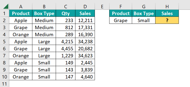
So, based on the changes done by the users, our formula should retrieve the value from the given column header name. To do this dynamically, we must include the MATCH function to get the column number for the column header given by the users.

We will use the previous formula, and remove the last bracket to find the column number.

Change the first index range from C2:C10 to C2:D10.

Now, to fetch the column number for the column header, enter the MATCH function.

Choose the lookup_value as cell H1.

Choose the table array from C1:D1.

Enter the matching type as an exact match, and close the bracket.

The formula returns the sales value because in cell H1, we have given the column header as “Sales”. Change the column name to “Quantity” to get the result from the quantity column.

Now the formula returns the values from the Quantity column.

Alternatives To INDEX MATCH Multiple Criteria

There are various alternatives to the INDEX MATCH multiple criteria. One such alternative is the combination formula of VLOOKUP and CHOOSE Excel functions.

Let us take the same data from the earlier example here as well.

First, let us understand how the CHOOSE function works.

For the CHOOSE function, we must enter the index number, and then it will choose the value from the respective position from the values given.

For instance, look at the following example.

In the Index argument, we have given 2, and in the values arguments, we have given days of the week.

There are 7 values (days) given, and the CHOOSE function chooses the value from the second position of the sequence of the values, i.e., “Tue”.

Similarly, we can combine all the lookup_value columns from the table, like the following.

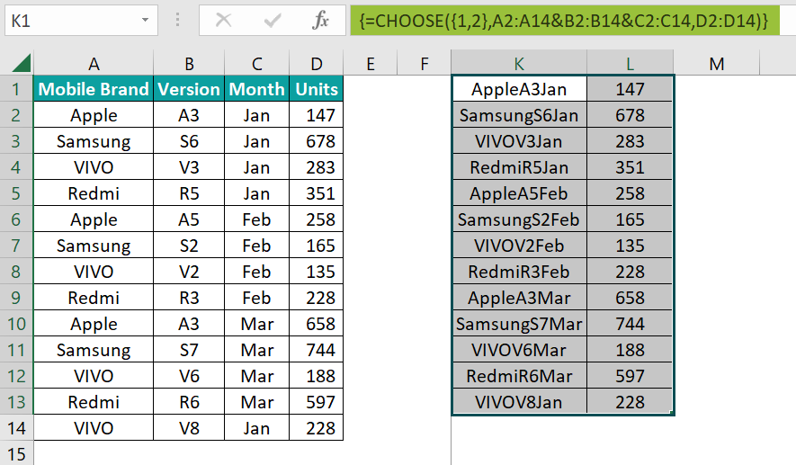
In the index number argument of the CHOOSE function, we have given 1 and 2 in the curly bracket, i.e., when we must select multiple values from multiple positions, we can use the curly bracket and mention the index numbers.

Then in the value1 argument, we have combined all the criteria columns, i.e., “Mobile Brand”, “Version”, and “Month” columns.

Then in the value2 argument, we have given reference to the “Units” column. Hence, the CHOOSE function returns the table, as shown below.

We can use the same formula in the table array argument of the VLOOKUP Excel function to avoid creating the helper column.

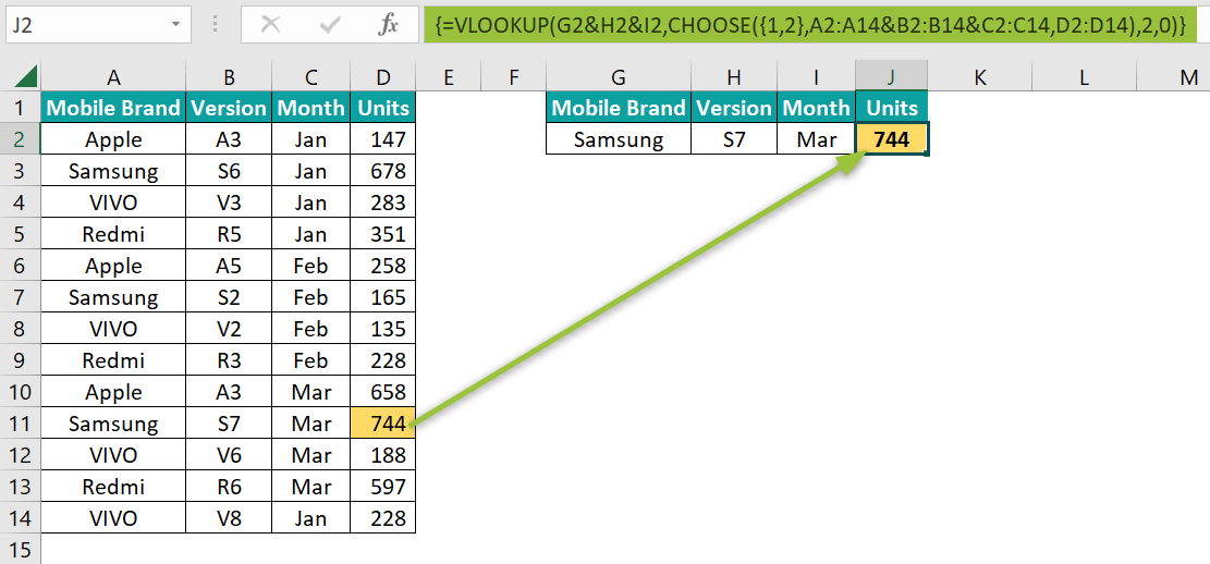
In the above formula, the CHOOSE function returns the table array as the concatenation of lookup_value columns and unit columns. Then, the VLOOKUP function retrieves the value from the table array given by the CHOOSE function.

Important Things To Note

• If we use Excel versions other than Office 365, we must execute all the formulas as an array formula using the keys Ctrl + Shift + Enter.
• The combination of VLOOKUP and CHOOSE is also an array formula in all the Excel versions apart from Office 365.
• The helper column method increases the size of the Excel workbook if you are working with a large data set.

Frequently Asked Questions (FAQs)

Download Template

This article must help understand INDEX MATCH multiple criteria with its formulas and examples. You can download the template here to use it instantly.

Recommended Articles

This has been a guide to INDEX MATCH Multiple Criteria. Here we find lookup value with INDEX-MATCH, VLOOKUP-CHOOSE, examples & downloadable excel template. You can learn more from the following articles –

• VLOOKUP with IF Statement
• VLOOKUP With SUM
• VLOOKUP to the Left