CHOOSE Function in Excel

What Is CHOOSE Function In Excel?

The CHOOSE function in Excel returns a value from an array based on a specified index number. It belongs to the category of Lookup & Reference functions. Users can use the Excel CHOOSE function when building scenarios in financial models. Also, it gives excellent results when combined with functions such as INDEX and VLOOKUP.

For example, consider the below image. The first table shows a list of car models, ranked by their sales figures.

Suppose we need to display the third-best-selling car in cell E1. Then, we can apply the Excel CHOOSE function in the target cell as depicted in the below image.

The CHOOSE function result in cell E1 shows the car model at the third position in the array of car models, as the index number mentioned in the function is 3.

What Is CHOOSE Function in Excel?

The CHOOSE() function returns a value from the value arguments based on the position of the value in the array.
Index_num and value1 are the mandatory arguments of CHOOSE(). While index_num can take a value from 1 to 254, we can supply a value of 1 to 254 to CHOOSE().
While the CHOOSE() function can be an alternative to nested IFs, we can use the function to generate random data and successfully do a left VLOOKUP.
When used with functions such as INDEX and MATCH, the CHOOSE() produces excellent results.

CHOOSE() Excel Formula

The CHOOSE Excel formula is:

where,

index_num: An integer that indicates the value argument. This argument must be any value from 1 to 254 or a cell reference to a cell having a number between 1-254.
value1, value2,…: The list of 1-254 values from which the CHOOSE function selects a value based on the specified index_num. They can be numbers, text, excel cell references, formulas, or text.

Below are a few aspects we must consider while using the CHOOSE function syntax.

If the index_num is 1, the CHOOSE() output will be value1. Likewise, if the index_num is 2, the CHOOSE function in excel result will be 2, and so on.
If the index_num argument is a fractional number, it gets truncated to the lowest integer.
If the index_num argument is an array, every array element gets assessed when the CHOOSE excel function gets evaluated.
If the index_num is a value below one or more than the number of entries in the value list, the function will return the #VALUE! error.
The value list contains individual values, cell references to cells containing the values, or cell range references, separated by commas.

While index_num and value1 are mandatory arguments, the rest are optional.

How To Use CHOOSE Excel Function?

The steps to use CHOOSE excel function are:

First, ensure we have the required arrays in the source data table.
Next, select the target cell and enter the CHOOSE() with the mandatory and required optional arguments.
Finally, press Enter to view the result.

Here is an CHOOSE function example to understand the steps.

Suppose we need to display the 6^th color in cell D2 from the list of colors in the first table, with cell D1 displaying the index value, 6, we need to use the following steps.

Step 1: First, select cell D2, type the below CHOOSE Excel function. Then, press Enter.

=CHOOSE(D1,A2,A3,A4,A5,A6,A7,A8,A9)

Alternatively, the above CHOOSE function example will work with the below formula:

=CHOOSE(6,”Red”,”Blue”,”Green”,”Yellow”,”Pink”,”Brown”,”Magenta”,”Orange”)

Here we directly provide the values as arguments to the CHOOSE() instead of entering the cell references to the values.

Likewise, we can use the Excel CHOOSE function to obtain the results.

Examples

Here are a few examples of how to use the Excel CHOOSE function.

Example 1 – CHOOSE As An Alternative To Nested IFs

Consider the below table. It shows the students’ aggregates and the grades legend.

Suppose we need to enter the grade for each student in column C, then we can use nested IFs with the below steps.

The formula in cell C2 would be:

=IF(B2>=91,$F$3,IF(B2>=76,$F$4,IF(B2>=61,$F$5,IF(B2>=46,$F$6,$F$7))))

And once we drag the Excel fill handle downwards to copy the nested IFs formula in cells C3:C11, the output will be:

However, we can use the CHOOSE function instead of the nested IFs function and make the formula more straightforward. The steps are:

Step 1: To begin with, select cell C2, and then, type the below CHOOSE(), and press Enter key.

=CHOOSE((B2<=45)+(B2<=60)+(B2<=75)+(B2<=90)+(B2<=100),$G$3,$G$4,$G$5,$G$6,$G$7)

Step 2: Next, drag the fill handle downwards to copy the formula in the cell range C3:C11.

In the above example, the Excel CHOOSE function multiple conditions define the index_num argument. Each condition will result in a 1 or 0, depending on whether the condition holds. And then, all the five results gets added to give the index_num value. On the other hand, the remaining arguments form the value list, containing five values.

For example, the calculations of CHOOSE Excel function with multiple conditions in cell C2 are:

=(0+0+0+0+1,$G$3,$G$4,$G$5,$G$6,$G$7)

=(1,$G$3,$G$4,$G$5,$G$6,$G$7)

Example 2 – Using CHOOSE With Arrays

Here is a table with three arrays, Book, TV Show, and Movie.

And suppose we need to update column E using the three arrays. Then we can use the CHOOSE excel function.

The steps used are as follows:

Step 1: First, select cell E2, type the below CHOOSE(), and press Enter.

=CHOOSE(2,A2:A7,B2:B7,C2:C7)

Step 2: Then, drag the fill handle downwards to copy the formula in the cell range E3:E7.

In the above example, each value in the value list is an array. And as the index_num is 2, the second array gets populated in column E.

Please Note: If you copy the formula in cells after cell E7, the cells will have a value of 0 as the second array in the source data in the range B2:B7.

Example 3 – Generate Random Data

If we require to generate random data, we can apply the Excel CHOOSE function, with the RANDBETWEEN() used as the index_num argument.

For example, the below table shows a list of players. We need to randomly allot a team, A, B, C, or D, to each of them with the following steps.

The steps used to obtain values with CHOOSE function are as follows:

Step 1: To begin with, select cell B2, type the below CHOOSE(), and press Enter key.

=CHOOSE(RANDBETWEEN(1,4),”TEAM A”,”TEAM B”,”TEAM C”,”TEAM D”)

Step 2: Drag the fill handle downwards to copy the formula in the range B3:B11.

There are four teams, TEAM A, TEAM B, TEAM C, and TEAM D. So, the index_num can be any value from 1 to 4.

The RANDBETWEEN() randomly generates an index number (between 1 to 4) every time the CHOOSE() executes. And depending on the generated index_num, the CHOOSE() returns the corresponding team name at the specific position in the supplied array.

Example 4 – CHOOSE Formula To Do A Left VLOOKUP

Consider the below table showing employee details.

Let us assume that we have to display the employee ID of an employee mentioned in cell F1 in cell F2. In such a scenario, a left VLOOKUP will not work; it will throw an error as shown in the following image.

Instead, we can apply the left VLOOKUP with the CHOOSE function in cell F2 to get the desired result.

Step 1: Select cell F2, type the below VLOOKUP function containing the CHOOSE(), and press Enter.

=VLOOKUP(F1,CHOOSE({1,3},C2:C7,B2:B7,A2:A7),2,0)

The term {1,3} ensures the columns A and C, EMP ID and Employee, get selected. And the CHOOSE() swaps the columns, making Employee and EMP ID columns the new columns A and B.

And since the CHOOSE() gives two columns as output, the VLOOKUP range becomes 2 instead of 3.

Example 5 – CHOOSE Function For Selecting Month

Let us assume that we need to enter the order month in column C in the below table.

Using the Excel CHOOSE function, we can enter the order months, deriving them from the dates in column B.

Step 1: First, select cell C2, type the CHOOSE() mentioned in the Formula Bar, and press Enter key.

Step 2: Next, drag the fill handle downwards to copy the formulas in range C3:C11.

The MONTH() is the index_num in the above CHOOSE(). It takes the date as the argument and returns the month number based on the date. Then the CHOOSE() returns the month name depending on the evaluated month number.

Thus, using the CHOOSE(), we can select months.

Things to Remember

The Excel CHOOSE function helps pick a value from an array of values, thus making it useful while selecting scenarios for developing powerful financial models.
The CHOOSE() will return the #VALUE! error if the index_num argument is not an integer or a cell reference to a numeric value. We might also see this error if the index_num is lesser than one or greater than the number of value arguments supplied to the function.
The CHOOSE() will return the #NAME? error if the value arguments are text values without double quotes or the cell references are invalid.

FAQs

When to use Excel CHOOSE function?

We can use CHOOSE function when we need a specific value from an array of values. We can apply the function when;

● Selecting a month.
● Using it as an alternative to nested IFs.
● Using it with RANDBETWEEN() to generate random data.
● Performing a left VLOOKUP.

Why use Excel CHOOSE function?

The Excel CHOOSE function can help us select a specific value from an array of 254 values, with the key benefit being that the function returns a value or a cell reference to the value.

On the other hand, creating scenarios is a critical step in developing financial models. The CHOOSE() enables us to select the required scenario from a set of scenarios according to your requirement.

How to use Excel CHOOSE function to return a custom day?

We can use CHOOSE excel function to return a custom day by following the below steps:

Consider the below table containing custom dates in column C.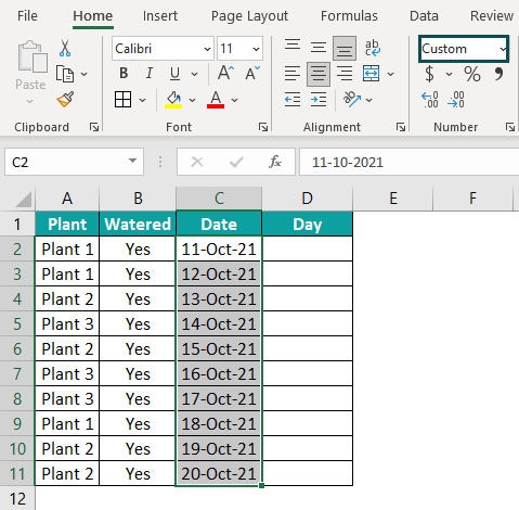

Excel CHOOSE Function FAQ 1

The steps to determine the custom day from the date in each cell, using the CHOOSE() are:

Step 1: Select cell D2, type the below CHOOSE(). Then, press Enter key.

=CHOOSE(WEEKDAY(C2),”Sunday”,”Monday”,”Tuesday”,”Wednesday”,”Thursday”,”Friday”,”Saturday”)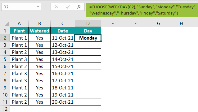

Excel CHOOSE Function FAQ 1.1

Step 2: Next, drag the fill handle downwards to copy the formula in the range D3:D11.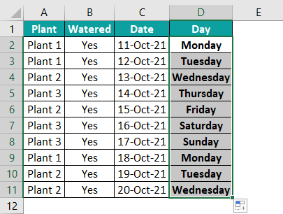

In the above example, the CHOOSE() contains custom days as the value arguments. The WEEKDAY() takes a date as an input and returns the day of the week as a number. The CHOOSE() considers the WEEKDAY() output as the index_num, based on which it returns the custom day for the specific date.

Download Template

This article must be helpful to understand the Excel CHOOSE Function, with its formula and examples. You can download the template here to use it instantly.

Excel CHOOSE Function Download