RANDBETWEEN Excel Formula

What Is RANDBETWEEN Formula In Excel?

The RANDBETWEEN formula in Excel returns a random integer between the range of any two specified numbers. And the function recalculates and returns a new random number every time the user opens or modifies the worksheet. The RANDBETWEEN Excel formula is an inbuilt Math & Trig function, so we can insert the formula from the “Function Library” or enter it directly in the worksheet.

For example, the table below contains a list of new employees. Here, we will generate employee IDs for the new employees using the RANDBETWEEN in Excel.

Select cell B2, enter the formula =RANDBETWEEN(100,200), press “Enter”, and drag the formula from cell B2 to B11 using the fill handle.

We get the output shown above. Here, we see that the new employee IDs are generated randomly between the two given numbers, 100 and 200.

What Is RANDBETWEEN Formula In Excel?

The RANDBETWEEN Excel formula results in generation of a random integer value between two given numbers. The function recalculates every time we open or update the worksheet.
We can use the RANDBETWEEN Excel formula to update a cell with a random number, and also to fill a cell range with random numbers. But for that, we must select the required cell range, type the RANDBETWEEN(), and press Ctrl + Enter to execute it.
While the function generates random integers, we can use it to fill cells with random decimal values, dates, and characters, using the functions such as INDEX, CHOOSE, DATE, DATEVALUE, CHAR, etc.

RANDBETWEEN() Formula Syntax

The syntax of the RANDBETWEEN Excel formula is,

The arguments of the RANDBETWEEN formula are,

bottom: The smallest integer in the range of random numbers needed. It will always be lesser than the top numeric value. It is a mandatory argument.
top: The largest integer in the range of random numbers needed. It can be any number greater than the bottom numeric value. It is a mandatory argument.

Excel VBA – All in One Courses Bundle (35+ Hours of Video Tutorials)

If you want to learn Excel and VBA professionally, then Excel VBA All in One Courses Bundle (35+ hours) is the perfect solution. Whether you’re a beginner or an experienced user, this bundle covers it all – from Basic Excel to Advanced Excel, Macros, Power Query, and VBA.

Start Learning Now

How To Use RANDBETWEEN Excel Formula?

We can use the RANDBETWEEN Excel formula in 2 ways, namely,

Access from the Excel ribbon.
Enter in the worksheet manually.

Method #1 – Access from the Excel ribbon

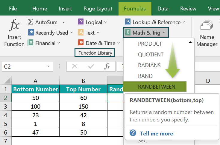
Choose an empty cell → select the “Formulas” tab → go to the “Function Library” group → click the “Math & Trig” option drop-down → select the “RANDBETWEEN” function, as shown below.

RANDBETWEEN Excel Formula - Access from the Excel ribbon

The “Function Arguments” window appears. Enter the argument values in the “Bottom”, and the “Top” fields → click “OK”, as shown below.

RANDBETWEEN Excel Formula - Function arguments window

Method #2 – Enter in the worksheet manually

First, ensure we have the two values required to generate the random number.
Then, select an empty cell for the output.
Type =RANDBETWEEN( in the cell. [Alternatively, type =R or =RA and double-click the RANDBETWEEN function from the Excel suggestions.]
Enter the arguments as cell values or excel cell references and close the brackets.
Finally, press Enter to execute the function.

Let us take a basic example to learn more about this function.

We will randomly generate numbers between the pairs of bottom and top numbers using RANDBETWEEN in Excel.

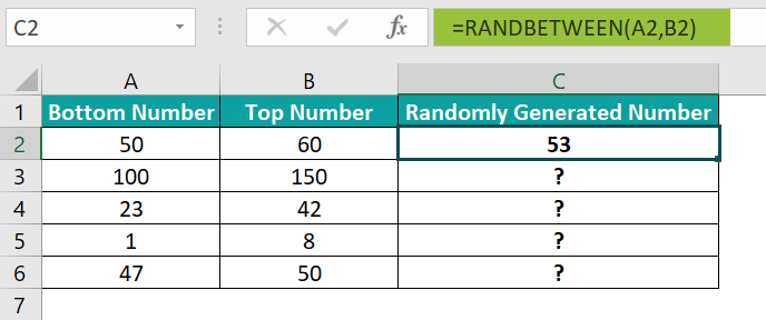
The following table contains a set of bottom and top numbers.

How to use RANDBETWEEN Function in Excel - Basic Example

The steps to generate random numbers using RANDBETWEEN Excel formula are,

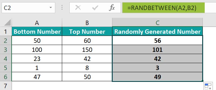
Select cell C2, enter the formula =RANDBETWEEN(A2,B2), and press Enter. The result is some random number between 50 and 60, here, 56.
Drag the formula from cell C2 to C6 using the fill handle.

We get the above result, i.e., the random numbers are generated in the selected cells between the number range of 50 to 60.

[Note: However, if we do not want the generated random numbers to update every time we make changes to the worksheet, then we can copy the values and paste them into the same column.]

[Alternatively, we can apply the RANDBETWEEN() from the Formulas tab. And for that, we can select the target cell and click Formulas → Math & Trig → RANDBETWEEN to open the Function Arguments window.

Next, enter the two RANDBETWEEN() argument values in the Function Arguments window.

And once we click OK in the Function Arguments window, a new random number will get generated in the target cell.]

Examples

We will understand some advanced scenarios with RANDBETWEEN Excel formula examples.

Example #1

We will display ten random numbers, for the following empty table, in the cell range A2:B6, between 250 and 300.

The steps to generate random numbers using RANDBETWEEN formula are,

Step 1: Select the cell range A2:B6, and enter the formula =RANDBETWEEN(250,300).

Step 2: Press Ctrl + Enter to execute the function.

We get the above output that shows the random number 279 repeated twice. It is not a RANDBETWEEN formula error, because if we require unique random numbers, double-click a target cell and recalculate the formula repeatedly till we get the desired outcome.

Step 3: Therefore, let us double-click cell B6, and press “Enter”, i.e., we are executing one of the formulas.

Step 4: Therefore, let us double-click cell B6, and press “Enter”, i.e., we are executing one of the formulas.And once we press Enter, all the cells with the RANDBETWEEN() get recalculated to give the below output with unique random numbers.

Example #2

We will generate random decimal numbers using the RANDBETWEEN formula.

The table below contains the minimum and maximum points one can score in each game round based on probability.

The steps to generate random scores using the RANDBETWEEN Excel formula are,

Step 1: Select cell D2, enter the formula =RANDBETWEEN(B2*100,C2*100)/100, and press Enter.

We get the result shown below.

Step 2: Drag the formula from cell D2 to D6 using the fill handle.

We get the output shown above.

[Output Observation: Let us consider the cell D6 formula to check how it works.

First, the cells B6 and C6 values get multiplied by 100. So, the bottom and top argument values become 25000 and 50000. Then the RANDBETWEEN() generates a random number between 25000 and 50000, 28412. Finally, the formula divides the randomly generated number 42544 by 100 to return the random decimal number 284.12.]

Example #3

We can use the RANDBETWEEN Excel formula to randomly get an order date in March from the source table.

The table below shows a list of products and their order dates.

The steps to generate random dates for March using the RANDBETWEEN formula with the INDEX Excel function are,

Step 1: Select cell D2, enter the formula =INDEX(A5:B8,RANDBETWEEN(1,4),2), and press Enter. We will get the following output.

Step 2: Select cell D2 and set the Number Format in the Home tab as Short Date to see the output as a date value.

Once we change the number format to date, we will get the required date, as shown below.

[Output Observation: In this example, the RANDBETWEEN() returns the random number 3, which lies between the specified bottom and top numbers 1 and 4. So, the INDEX() takes the RANDBETWEEN() output, 3, as the row_num argument value, and the column_num is 2. And thus, the INDEX() returns the date in the specified cell reference, row 3 and column 2, in the given cell range A5:B8, 20-03-2022.]

Example #4

We can use the RANDBETWEEN formula to generate random letters using CODE() and CHAR Excel function to assign a team to each player, with the teams being A, B, C, and D.

The below table contains a list of players.

The steps to use the RANDBETWEEN Excel formula with the CHAR() and CODE() are,

Step 1: Select cell B2, enter the formula=CHAR(RANDBETWEEN(CODE(“A”),CODE(“D”))), and press Enter.

Step 2: Drag the formula from cell B2 to B11 using the fill handle.

We get the above-generated letters.

[Output Observation: The first CODE() returns the code of the letter A, 65, and the second one returns the code of the letter D, 68. Next, the RANDBETWEEN() returns a random number between 65 and 68, which the CHAR() returns as the corresponding letter.

As the bottom and top arguments limit the codes between 65 to 68, the CHAR() returns letters between A to D, the required teams.]

Important Things To Note

If we do not want the RANDBETWEEN() to recalculate, we can select the cell containing the function and press Ctrl + C to copy the cell content. And then, we can press the shortcut keys Alt + E + S + V to paste special as a value. We can also double-click the cell containing the RANDBETWEEN() or click the Formula Bar and press F9 as an alternative.
Sometimes the function might generate repetitive random numbers in multiple cells. Please do not consider it as a RANDBETWEEN Excel formula error. We can recalculate the function multiple times till we get unique random values.
Ensure the bottom argument value is less than the top argument value. Otherwise, the RANDBETWEEN() output will be the #NUM! error.
For incorrect argument data type, the RANDBETWEEN() returns the #VALUE! error.

Frequently Asked Questions (FAQs)

1. How to use the RANDBETWEEN Excel formula to generate random dates?

We can use the RANDBETWEEN Excel formula to generate random dates with the help of the Excel functions DATE or DATEVALUE.

For example, we will update the table with six random dates between 10/1/2022 and 10/20/2022.

The steps to use the RANDBETWEEN() with the DATEVALUE() are,

• Step 1: Select the target cell range A2:F2 and set the Number Format in the Home tab as Short Date to view the output as date values.

• Step 2: Select the target cell range A2:F2, enter the formula =RANDBETWEEN(DATEVALUE(“1-Oct-2022”),DATEVALUE(“20-Oct-2022”)), and press Ctrl + Enter, as shown below.

We get the generated random dates as shown below.

The DATEVALUE() returns the serial number of the respective supplied dates. So thus, the RANDBETWEEN() returns six random dates between the specified date values in the six selected target cells.

2. Why is the RANDBETWEEN Excel formula not working?

The RANDBETWEEN Excel formula is not working, perhaps because of the following reasons:
• The supplied bottom argument value is more than the provided top argument value.
• The supplied arguments have the wrong data type.

3. Can we generate random numbers with no duplicates using the RANDBETWEEN Excel formula?

We can generate random numbers with no duplicates using the RANDBETWEEN Excel formula with the RANK.EQ and COUNTIF functions.

For example, we must generate ten random numbers between 20 and 50.

• Step 1: First, to apply the RANDBETWEEN(), select the cell range A2:A11, enter the formula =RANDBETWEEN(20,50), and press Ctrl + Enter to execute the function.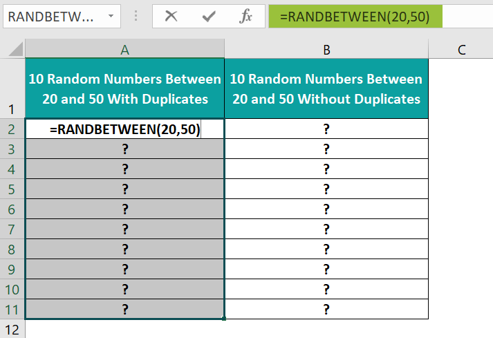

The random number 22 appears thrice in the output, as shown below.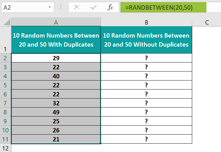

• Step 2: To avoid getting duplicate numbers, select cell range A2:A11, press Ctrl + C, and then Alt + E + S + V to copy and paste special the values. Choose from the “Paste Special” window, as shown.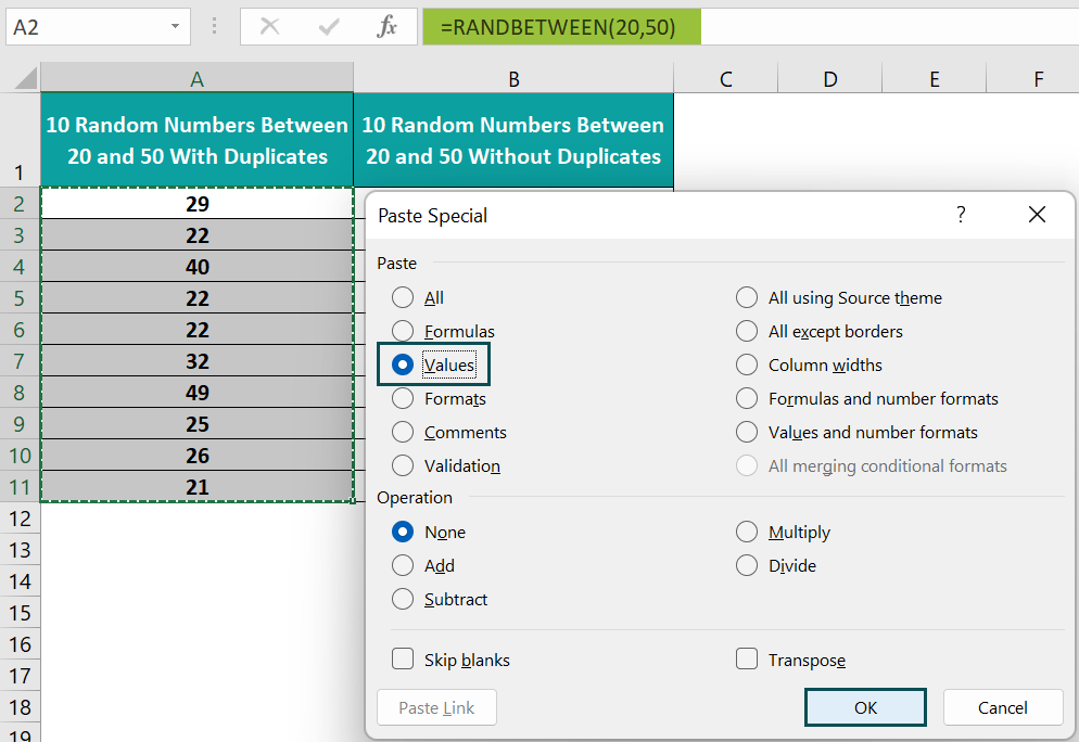

And once we click OK, we will see the values in the Formula Bar instead of the formulas.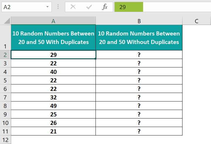

• Step 3: Select cell B2, enter the formula=19+RANK.EQ(A2,$A$2:$A$11)+COUNTIF($A$2:A2,A2)-1, and press Enter.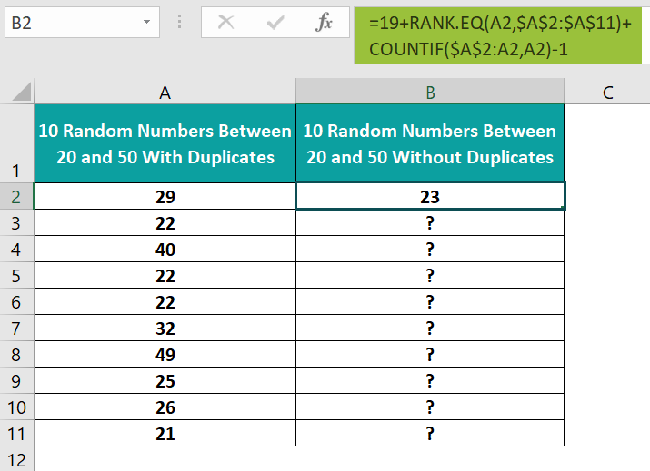

• Step 4: Drag the formula from cell B2 to B11 using the fill handle.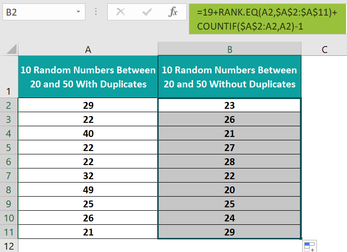

[Output Observation: Let us consider the cell B11 formula to see how it works. First, as the bottom argument value is 20, we add 19 to the result. Then the RANK.EQ() returns the rank of value 21 in the cell range A2:A11, as 10, with the ranking in descending order. And as the value 21 occurs once in the cell range A2:A11, the COUNTIF() returns the count as 1. Thus, the formula simplifies to return the value 24 (19+10+1-1).

In the case of the value 22, in row 3, the COUNTIF() returns 1. But, on the other hand, as the value appears again in rows 5 & 6, the COUNTIF() in the cell B6 formula returns 3. So, with the RANK.EQ() returning the same rank, 7, for the value 22, the formula returns unique values in rows 3, 5 and 6 target cells, B3, B5 and B6. Thus, in this way, we achieve a list of random numbers without duplicates.]

Download Template

This article must help understand the RANDBETWEEN Excel Formula, with its formula and examples. We can download the template here to use it instantly.

RANDBETWEEN Excel Formula Download

RANDBETWEEN Excel Formula