What Is RAND Function In Excel?
The RAND function in Excel creates evenly distributed random real numbers. These generated random values are between 0 and 1, so the values range is greater than or equal to 0 and less than 1.
The RAND Excel Function is a Volatile function. So, the values are recalculated every time the worksheet is opened or modified, or the calculation is prompted. As a result, the random numbers generated in the selected cells are unique and are not repeated in the same selection.
For example, we apply the RAND Function to calculate random numbers in cell A1.
Enter the formula =RAND(), and press the “Enter” key.
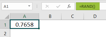
The output is “0.7658”, as shown above. A random number is generated between 0 and 1 without getting any input in the formula.
📥Download the ready-to-use Excel template to practice this tutorial yourself.
RAND Excel FunctionTable of contents
Key Takeaways
- The RAND Excel function generates random numbers from 0 to 1. It can also generate random percentages from 0% to 100%.
- Since it is a Volatile function, it generates a new value each time the worksheet is opened, or the formula is triggered.
- To calculate the random numbers between two numbers, we must use the following RAND formula, “=a+ (b-a)*RAND ()”. [a and b can be any integers].
- We can use the RAND Function and change the output cell format to “Time” to generate random time, just like random numbers.
RAND() Excel Formula
The Syntax of the RAND Excel formula is,
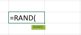
The formula does not have any arguments.
How To Use RAND Excel Function?
The RAND Excel function can be used in 2 methods, namely,
- Access from the Excel ribbon.
- Enter the worksheet manually.
#1 – Access From the Excel Ribbon
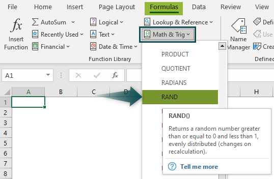
Choose an empty cell for the result > select the “Formulas” tab > go to the “Function Library” group > click the “Math & Trig” drop-down > select the “Rand” function option, as shown below.
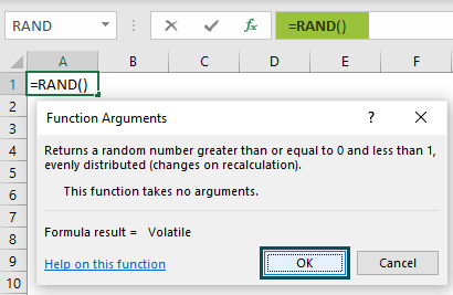
The RAND Excel formula is inserted in the cell, and the “Function Arguments” window instantly appears, as shown below. Since this function has no arguments, click “OK”.
#2 – Enter the Worksheet Manually
- Select an empty cell for the output.
- Type =RAND() in the selected cell. [Alternatively, type “=R” and double-click the RAND function from the list of suggestions shown by Excel].
- Press the “Enter” key.
# Basic Example
We will generate random numbers using the RAND Excel formula.
In the table, the data is,
- Column A contains the Output to be calculated.
- Column B contains the Formula for our reference.
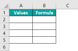
The steps to generate the random numbers using the RAND Function are as follows:
Step 1: Select cell A2, enter the formula =RAND() and press the “Enter” key. The output is ‘0.274’, as shown below.
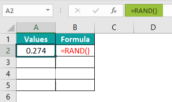
Step 2: Drag the formula from cell A2 to cell A5 using the fill handle.
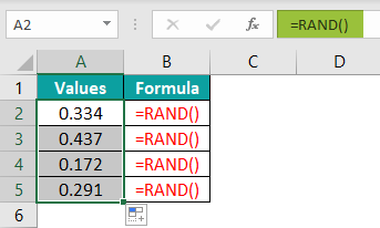
The output is shown above. The formulas displayed in Column B are for our reference.
[Note: The RAND function generates random numbers between 0 and 1, so the above example returns random numbers between 0 and 1].
Examples
We will understand the RAND in Excel with some advanced scenarios.
Example #1
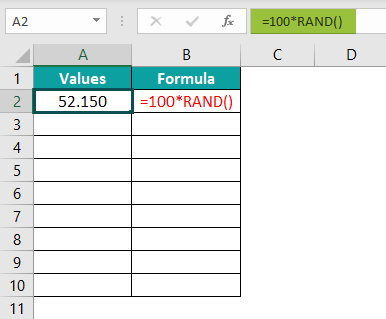
We will generate random numbers between 0 and 100 using RAND Excel Function.
In the table, the data is,
- Column A contains the Output to be calculated.
- Column B contains the Formula for our reference.
The steps to generate the random numbers using the RAND in Excel are as follows:
Step 1: Select cell A2, enter the formula =100*RAND() and press the “Enter” key. The output is ‘52.150’, as shown below.
Step 2: Drag the formula from cell A2 to cell A10 using the fill handle.
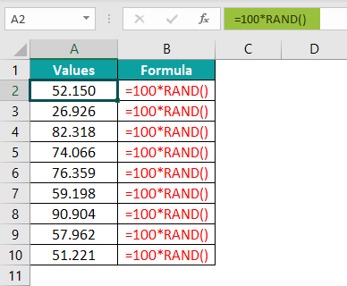
The output is shown above. The formula =100*RAND() first generates the random numbers between 0 and 1, multiplies the result by 100, and returns the output between 0 and 100.
[Note: The RAND Excel function generates random numbers only between 0 and 1. However, we can build formulas like the above example and generate random numbers between different numbers].
Example #2
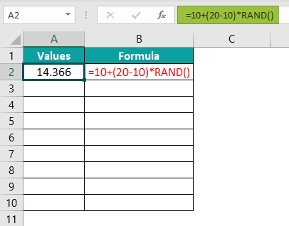
We will generate the random number between 10 and 20 using RAND Function. In this example, the formula used is “=a+(b-a)*RAND()”. When we enter the two values, 10 and 20, the formula will then be “=10+(20-10)*RAND()”.
In the table, the data is,
- Column A contains the Output to be calculated.
- Column B contains the Formula for our reference.

The steps to generate the random numbers using the RAND Excel function are as follows:
Step 1: Select cell A2, enter the formula =10+(20-10)*RAND() and press the “Enter” key. The output is ‘14.366’, as shown below.
Step 2: Drag the formula from cell A2 to cell A10 using the fill handle.
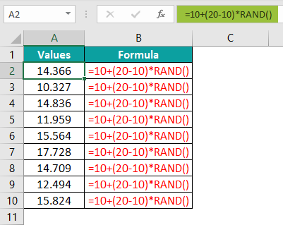
The output is shown above.
[Note: Using the formula =a+ (b-a)*RAND(), the RAND Excel Function generates the random number between two integers, 10 and 20, as seen in the above example]
Example #3
We will generate random time using RAND Excel Function.
In the table, the data is,
- Column A contains the Output to be calculated.
- Column B contains the Formula for our reference.
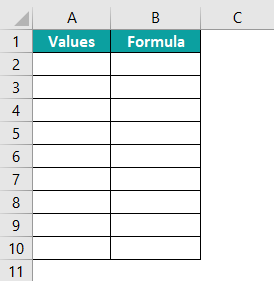
The steps to generate the random time using the RAND Excel function are as follows:
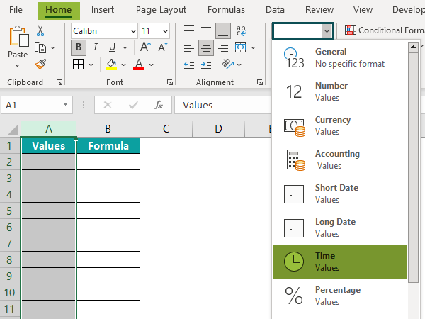
Step 1: First, we will set column A to “Time” format. Choose column A > select the “Home” tab > go to the “Number” group > click the “Number Format” drop-down > select the “Time” option, as shown below.
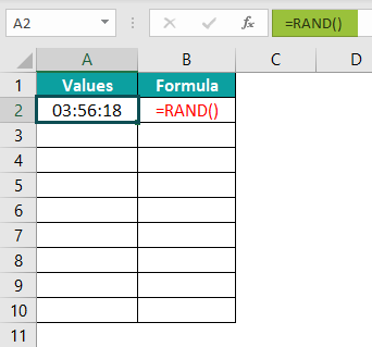
Step 2: Enter the formula =RAND() in cell A2 and press the “Enter” key. The output is ‘06:34:05’, as shown below.
Step 3: Drag the formula in cell A2 to cell A10 using the fill handle.
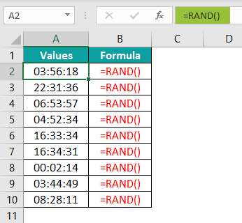
The output is shown above in the “Time” format.
Important Things to Note
- The RAND Excel function reduces the speed of the workbook due to consistent recalculation of the randomly generated values.
- To generate a set of random numbers in multiple cells, instead of dragging the formula, first, select the cell range for the output, enter the RAND() formula, and then press the “CTRL+ENTER” keys in place of the “Enter” key.
- To stop the auto-change in the RAND Excel function, click on the result that we do not want to change. Then, in the Formula Bar, press the F9 key [in some cases, Fn+F9] to convert the formula into its value.

Frequently Asked Questions (FAQs)
The purpose of the RAND function in Excel is as follows:
1. The RAND or RANDBETWEEN function in Excel generates a list of random numbers. It creates more values than we need, and we can delete some duplicates later.
2. We can convert formulas to values to prevent Excel random functions from recalculating.
3. The function removes duplicate values using Excel’s built-in tool or the advanced Duplicate Remover for Excel.
We can use the RAND function works in Excel as follows:
1. Select an empty cell to enter the Formula.
2. Type =RAND() in the selected cell. [Alternatively, type “=R” and double-click the RAND function from the list of suggestions shown by Excel].
3. Press the “Enter” key.
Let us generate random numbers using the RAND Excel Function for the following example, where
Column A contains the Output to be generated.
The procedure to use RAND Excel Function is,
Select cell A1, enter the formula =RAND(), and press the “Enter” key. The result in cell A1 is ‘0.4072’. Now, drag the formula to cell A2 using the fill handle. The output is shown below.
We can find the RAND function using the following steps:
Choose an empty cell for the result > select the “Formulas” tab > go to the “Function Library” group > click the “Math & Trig” drop-down > select the “Rand” function option, as shown below.
The RAND Excel formula is inserted in the cell, and the “Function Arguments” window instantly appears, as shown below. Since this function has no arguments, click “OK”.
Download Template
📥Download the ready-to-use Excel template to practice this tutorial yourself.
RAND Excel FunctionRecommended Articles
This has been a guide to RAND Excel Function. Here we get random numbers from 0 to 1, other values by built formulas, examples & downloadable excel template. You can learn more from the following articles –

Leave a Reply