MID Excel Function

What Is MID Function In Excel?

The MID Excel function returns a specified number of characters from the middle of a given text string. Also, the MID function can be used with VALUE, SUM, COUNT, DATE, DAY, and other functions. The MID Excel function is available under the Excel TEXT functions group.

For example, the below table shows the value in cell A2. Now, we need to apply MID function to detect the output.

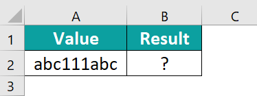
The steps used to apply MID excel function are as follows.
To begin with, select the cell to display the output. In our example, the cell is B2.
Next, enter the complete formula =MID(A2,4,3)Then, press Enter key.
The function has returned the output as shown in the below image.

Likewise, we can apply MID function to obtain the middle value.

What is MID Function in Excel?

The syntax of the MID excel function is =MID(text,start_num,num_chars) where,
- text denotes the original text string.
- start_num indicates the integer that specifies the position of the first character we want to be returned.
- num_chars shows the number of characters, starting with start_num, to be returned from the start of the text. It is the number of characters to be extracted.

If the user does not specify the last parameter of the MID function, it will take 0 by default.
The number formatting is not the part of a string and cannot be extracted or counted.

MID() Excel Formula

The syntax of the MID excel formula is:

where,

text: It denotes the original text string.
start_num: It indicates the integer specifying the position of the first character we want to be returned.
num_chars: It shows the number of characters, starting with start_num, to be returned from the start of the text. It is the number of characters to be extracted.

Unlike other functions, all the arguments are mandatory in MID excel formula.

Excel VBA – All in One Courses Bundle (35+ Hours of Video Tutorials)

If you want to learn Excel and VBA professionally, then Excel VBA All in One Courses Bundle (35+ hours) is the perfect solution. Whether you’re a beginner or an experienced user, this bundle covers it all – from Basic Excel to Advanced Excel, Macros, Power Query, and VBA.

Start Learning Now

How To Use MID Excel Function? (With Steps)

#1 – Access From The Excel Ribbon

Choose the empty cell to display the result.
Go to the Formulas tab.
Select Text from the menu.
Select MID from the drop-down menu.
The Function Arguments window appears.
Based on the number of arguments, enter the value in the Text, Start_num, and Num_chars.
Select OK.

#2 – Enter The Worksheet Manually

Select an empty cell for the output.
Type =MID( in the selected cell. Alternatively, type =M and double-click the MID function from the list of suggestions shown by Excel.
Enter the arguments as cell references or direct values.
Close the parenthesis and press the Enter key.

Let us take a basic example to understand this function. The following table shows the strings in column A. Now, we need to extract the text from the string using MID excel function.

The steps to extract the text from the string using MID Excel function are as follows:

To begin with, select the column to display the result. The selected column, in this case, is column B.
Next, enter the MID excel function formula in cell B2.
Select the cell A2 in the text argument.

Enter the value as 10 in the start_num argument.

Enter the value ‘4’ in the num_chars argument.

So, the complete formula is =MID(A2,10,4).
Then, press Enter key.
We can see that the function has returned ‘boat’ in cell B2.
Drag the cursor to cell B5 using AutoFill option.

Likewise, we can use MID function to extract mid values.

Examples

Example #1 – Extracts The First And Last Names From The Full Names

The below table shows the full name of various people in column A. We need to extract the first name and the last name from the given table array using MID Excel function.

The steps to extract the text from the string by the MID in Excel are as follows:

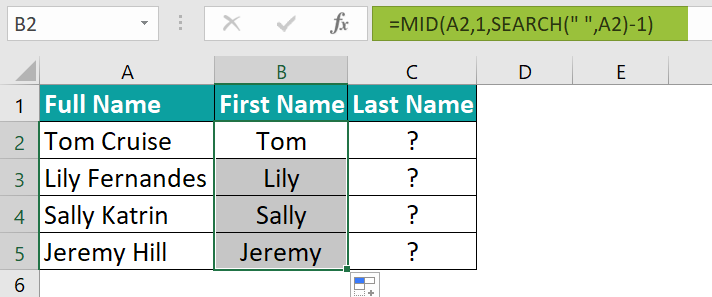
Step 1: To begin with, select the column to display the cell. In this example, we will enter the First name in column B and the Last name in column C.

Step 2: Next, enter the MID formula in cell B2 for extracting the first name.

Step 3: Now, enter the value for the text argument as A2.

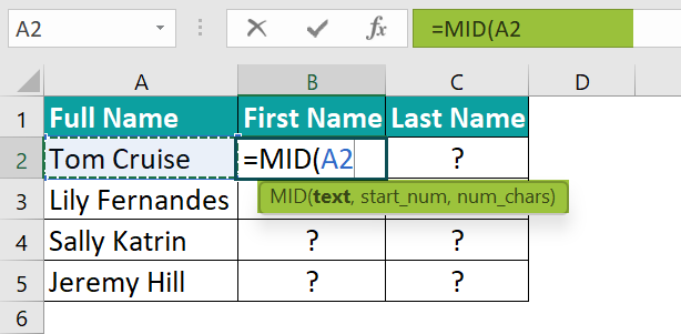
Step 4: The value entered for the start_num argument is 1.

Step 5: The value entered for num_chars argument is the SEARCH formula as we extract the first name.

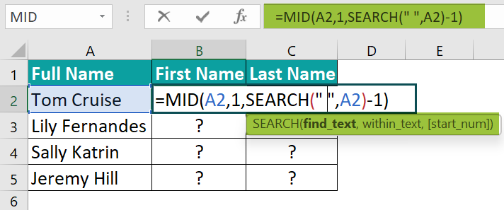
Step 6: The entered complete formula in cell B2 for extracting the first name is =MID(A2,1,SEARCH(“ ”,A2)-1)

Press Enter key.

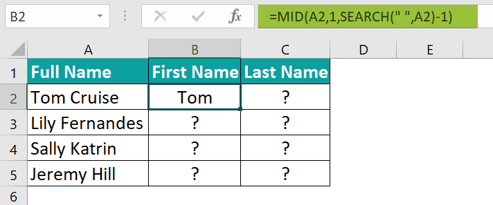
Step 7: The result is returned as Tom.

Next, drag the cursor to cell B5; all the first name from the data is extracted in column B as shown in the following image.

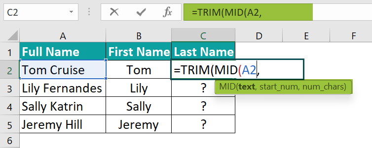
Step 8: Next, enter the MID formula in cell C2 for extracting the Last name.

Step 9: Firstly, we will enter the TRIM Excel formula, and then the MID formula value entered for the text argument is A2.

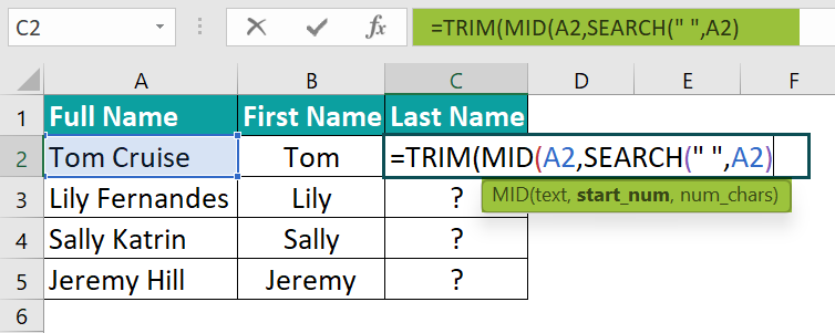
Step 10: Now, enter the value for the start_num argument and the SEARCH formula for extracting the last name.

Step 11: The value entered for the num_chars argument is the LEN excel formula as we are extracting the Last name.

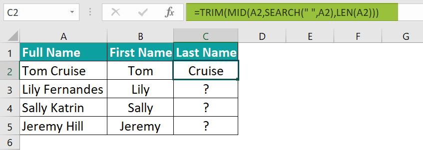
Step 12: So, the entered complete formula in cell C2 for extracting the last name is =TRIM(MID(A2,SEARCH(“ ”,A2),LEN(A2)))

Press Enter key.

The result is returned as Cruise.

Step 13: Drag the cursor to cell C5;

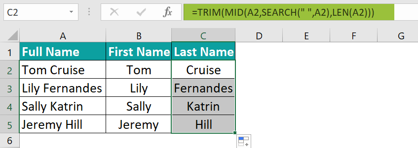
Likewise, we can use MID Function to extract values.

Example #2 – Find Out The Domain Name From The Web URLs

The below table shows the Web URLs in column A. We need to use the following steps to find the domain name from the table array using MID Excel Function.

The steps to extract the text from the string by the MID in Excel are as follows:

Step 1: To begin with, select the column where we will enter the formula and calculate the result. The selected column, in this case, is column B.

Step 2: Next, enter the MID Excel formula in cell B2 for extracting the domain name.

Step 3: The complete formula in cell B2 for extracting the domain name is =MID(A2,SEARCH(“://”,A2)+3,SEARCH(“/”,A2,SEARCH(“://”,A2)+3)-SEARCH(“://”,A2)-3).

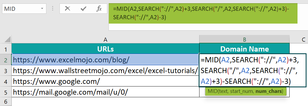
Step 4: The result is returned as www.excelmojo.com in cell B2.

Step 5: Now, drag the cursor to cell B5; all the domain name from the data is extracted in column B.

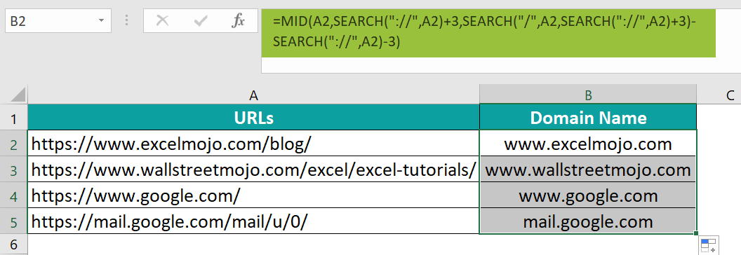
Similarly, we can use MID function to find the values.

Example #3 – Extracting Last n Digits From Some Numbers

The following table shows numbers in column A. We need to extract the last n digits from the given data using MID Excel function.

The steps to extract the text from the string by the MID Excel function are as follows:

Step 1: First, select the column where we will enter the formula and calculate the result. The selected column, in this case, is column B.

Step 2: Next, enter the MID formula in cell B2 for extracting the Last n Digits.

Step 3: So, the complete formula in cell B2 for extracting the Last n Digits is =MID(A2,LEN(A2)-2+1,2).

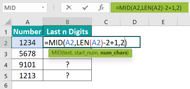
Step 4: The function has returned the result as 34 in cell B2.

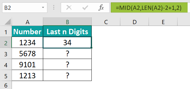
Step 5: Next, press Enter and drag the cursor to cell B5;

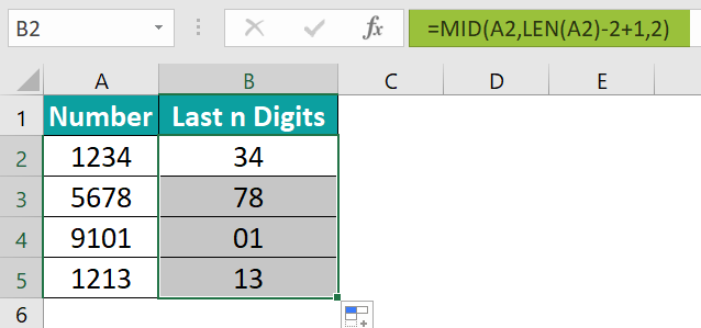
Likewise, we can use MID excel function to obtain the values.

Example #4 – MID Function With Arrays

The following table shows input values of fruits in column A. We need to extract the text from the table array using MID Excel function.

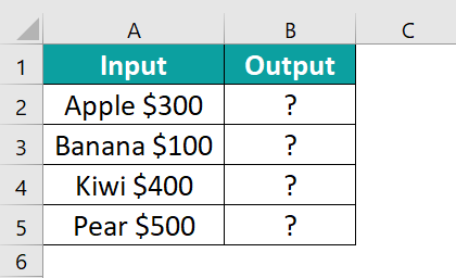
The steps to extract the text from the string by the MID in Excel are as follows:

Step 1: First, select the column where we will enter the formula and calculate the result. The selected column, in this case, is column B.

Step 2: Next, enter the MID formula in cell B2 for extracting the data from the array.

Step 3: Then, enter the value for the text argument as A2:A5.

Step 4: Similarly, enter the value for the start_num argument as 1.

Step 5: The value entered for the num_chars argument is the SEARCH formula as we extract the text.

Step 6: The entered complete formula in cell B2 for extracting is =MID(A2:A5,1,SEARCH(“ ”,A2:A5)).

We can see that the function has returned the value in B2.

Step 7: Drag the cursor to cell B5;

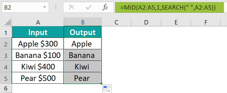
Similarly, we can use MID Excel function to find values.

Things To Remember

The MID Excel function returns the middle or central characters in the data.
The MID function is used in conjunction with VALUE, SUM, COUNT, DATE, DAY, and other functions.
All the arguments in MID Excel formula are mandatory.
The function extracts the characters from any side of a specified text.
It extracts text from inside a text string based on location and length.
The MID function returns empty text if the start_num is greater than the length of a string.
The “#VALUE!” error occurs if the value of the num_chars argument is less than 0 or if the value of the start_num argument is less than 1.

Frequently Asked Questions (FAQs)

1. What does the MID function do in Excel?

The MID function extracts the substring from the main string.
The syntax of MID is
=MID(text,start_num,num_chars)
For example, the below table shows the value in cell A2. We need to apply MID Excel function to detect the output.

The MID formula is entered in cell B2; the complete formula is =MID(A2,4,3),and the result is returned as 456.

FAQ1-1

Likewise, we can apply MID Excel function to obtain values.

2. When to use the MID Excel function?

The MID Excel function is used when we want to extract a small amount of data from huge data. That is when we want to fetch the text or number from a string or bunch of numbers.

3. Why does the MID function not work in Excel?

The MID function does not work in Excel due to two reasons;
1. If the value is equal to ‘0,’ the MID function will return a blank cell.
2. If the value is less than ‘0,’ the MID function will return “#VALUE!”.

Download Template

This article must help understand MID in Excel with its formula and examples. You can download the template here to use it instantly.

MID Excel Function Download

MID Excel Function