
What Is TRIM Excel Formula?
TRIM in Excel removes all extra spaces from the data or text except single spaces between words. It was designed to trim the 7-bit ASCII space character (value 32) from the data or text. Also, the TRIM formula in Excel – TRIM() trims the irregular spacing between strings.
For example, in the following image, alphabets are shown, but with extra spaces in between. The TRIM formula in Excel will trim extra spaces except for one space between alphabets, as shown below:
Use this TRIM In Excel Template to follow along with the examples in this article.
Download Excel Template=TRIM(A2)

The results in all B2 and B3 are as follows:
- AB
- CDE

Key Takeaways
- The TRIM function is used to remove irregular text spaces and retain single spaces between words in Excel. Irregular text spaces are unnecessary spacing that occur before, between or after text and numbers.
- The syntax of text is =TRIM(text). Here, text is the string or number from which spaces are to be removed.
- It is useful in finance in removing spaces in data from third-party applications.
- TRIM cannot remove Unicode text with a non-breaking space character (160).
TRIM() Formula In Excel

- text= It refers to the text from which extra spaces are required to be removed. It is the mandatory argument of the TRIM formula in Excel.
How To Use TRIM In Excel?
Below is the step by step representation of the TRIM formula in Excel, i.e., =TRIM(text):
- Select the cell where to enter the formula.
- Type =TRIM in the cell.
- Open brackets and select cells which are to be trim in the text.
- Close brackets and press ‘Enter.’
Examples
Let us look at some TRIM in Excel examples to understand the formula:
Example #1 (Basic)
The following excel image shows the people’s names written in the wrong format:

Here, the TRIM function will trim the extra spaces between words. In the table below, the data reflect the following:
Column A contains the names of the people
Column B trims the string
Step 1: The TRIM function eliminates spaces between the words, except for a single space between words. For doing this, enter the following TRIM formula in Excel in cell B2:
=TRIM(A2)

Step 2: After inserting the formula in cell B2, you may receive the result as, “Wiliam (SPACE) (SPACE) (except single SPACE) Citrus.”

Step 3: Press the “Enter” key. Then, drag the formula downwards till cell B4.
The result in all cells may display as follows:
- Wiliam Citrus
- Jack Hill
- Elion Musk

Example #2 (Trim White Spaces In Excel)
The following image shows the list of incorrectly written idioms, with extra white spaces between words:

Using the TRIM in Excel, we can trim the extra white spaces between words.
In the given table, the data displays the following:
Column A contains the list of Idioms
Column B trims the text
Step 1: The Excel function TRIM removes spaces between the words, except for a single space between words. For using this function, enter the following TRIM formula in Excel in cell B2:
=TRIM(A2)

Step 2: Next, after inserting the formula in cell B2, the result may come as “Under (WHITE SPACE) (WHITE SPACE) (except single SPACE) the (WHITE SPACE) (WHITE SPACE) (except single SPACE) weather.”

Step 3: Press the “Enter” key. Then, drag the formula downwards till cell B8.
As a result, it will display the following data in all cells:
- Under the weather
- Spill the beans
- Through thick and thin
- Take it with a pinch of Salt
- Go down in Flames
- Jump on the bandwagon
- As right as rain

Example #3 (Using TRIM Function With SUBSTITUTE Function)
The following image shows the phone numbers but with spaces in between, but in various manners, like at the beginning of the number, middle of the number, and end of the numbers. The TRIM and SUBSTITUTE functions in Excel will trim the extra spaces between numbers:

The SUBSTITUTE function in Excel helps us replace specific text in a text string.
The syntax of the SUBSTITUTE function is:
=SUBSTITUTE(text,old_text,new_text,[instance_num])
- text = the text string which needs to be substituted
- old_text = the old text string which needs to be replaced
- new_text = the new text to be used as a replacement
- instance_num = specify the occurrence of old text replaced with new text
In this example, the SUBSTITUTE function is used with the TRIM function to eliminate the non-breaking space in the phone numbers.
The TRIM function considers numbers as text, eliminating the extra spaces between numbers except for a single space. The SUBSTITUTE function substitutes single spaces with no space in between the numbers.
In the table, the data is reflected as below:
Column A contains the phone numbers which are to be trimmed
Column B trims contents
Step 1: The TRIM function eliminates spaces between the numbers but cannot trim a single space, so the SUBSTITUTE function is used. The following TRIM and SUBSTITUTE formulas in Excel is entered in cell B2.
=TRIM(SUBSTITUTE(A2,” “,””))

Step 2: The result comes as “954 (SPACE) 567877 (SPACE) 2”.

Step 3: Press the “Enter” key. Drag the formula downwards till cell B8.
The results in all cells are as follows:
- 9545678772
- 9023346785
- 9837732738
- 7786787796
- 7453454566
- 8956675668
- 9767635667

Therefore, the SUBSTITUTE function with the TRIM function proves better than the alone TRIM function when removing spaces between numbers.
Example #4 (Remove Extra Spaces Between Different Text Formats)
The following image displays the different text formats but with spaces in between. For example, there are alphabets, numbers, sentences, dates, and names with spaces in between in various manners, like at the beginning of the text, middle of the text, and end.

Using the TRIM in Excel, we may trim the extra spaces between words and numbers.
In the table, the data reflect the following:
Column A contains the contents which are to be trimmed
Column B trims contents
Step 1: This TRIM function eliminates spaces between the texts, except for a single space between words and no spaces between single characters and numbers. To use this function, enter the following TRIM formula in Excel in cell B2:
=TRIM(A2)

Step 2: After entering the formula is entered in cell B2. You may receive the result as “A (SPACE) B (SPACE) C (SPACE) (SPACE) D.”

Step 3: Press the “Enter” key. Then, drag the formula downwards till cell B9.
As a final result, you may view the following in all cells:
- ABCD
- 1234
- TRIM function in Excel
- 1111
- 2222
- More and More Space
- 29 / 03/ 2022
- Denis Richard

Important Things To Note
- TRIM in Excel removes extra spaces from the text and leaves only a single space between words
- It only removes ASCII space character (32) from text or string.
- Remember, you may also use this Excel function for cleaning text from other applications or environments.
- TRIM cannot remove Unicode text with a non-breaking space character (160) visible in the form of the HTML entity on web pages.
- The TRIM function does not eliminate one space character known as non-breaking space.
- To eliminate the non-breaking space, use the SUBSTITUTE function, which replaces all non-breaking spaces between words with regular spaces, and the CHAR function, which requires the relevant ASCII code for the two different spaces into the formula – 160 & 32 in the place of the TRIM function.
- The SUBSTITUTE function is used for changing any ASCII code with any other code.
- If you want to remove all spaces in the data from the Excel sheet, use the ‘Find & Replace’ feature.
- When text is used in calculations or data validation, the TRIM function is crucial because spaces before and after the text are significant.
Frequently Asked Questions (FAQs)
Follow the below steps to execute the TRIM function in Excel, i.e., =TRIM(text):
1. Select the cell to enter the formula.
2. Type =TRIM in the cell.
3. Then, select the cells which are needed to be trimmed.
4. Close the brackets and press the “Enter” key.
For example, the following image lists company names but extra spaces between alphabets. With the use of the TRIM function, we can remove the spaces.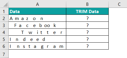
The following TRIM formula in Excel will trim extra spaces between and before the numbers.
=TRIM(A2)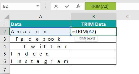
The results in all cells are as follows:
1. Amazon
2. Facebook
3. Twitter
4. Indeed
5. Instagram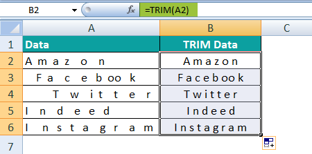
The following example explains how to TRIM data in Excel. The data is in numeric form. In the following image, numbers are shown with extra spaces.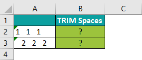
With the help of the given-below TRIM formula in Excel, we can trim extra spaces between and before the numbers.
=TRIM(A2)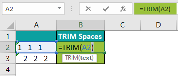
The results in all cells are as follows:
1. 111
2. 222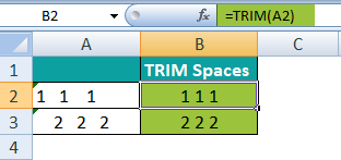
TRIM formula in Excel is as follows:
=TRIM(text)
1. The TRIM in Excel discards all spaces (excluding single spaces) from the data or text.
2. The TRIM on text can be done when received from other applications.
3. The TRIM function removes the unwanted spaces between the words or from the beginning or end of the words.
4. The function eliminates the 7-bit ASCII space characters from the text.
Use this TRIM In Excel Template to follow along with the examples in this article.
Download Excel TemplateRecommended Articles
Continue with these related resources when you want the next practical step in this topic.
- TEXT Function In Excel
- LEN Excel Function
- LEFT Function in Excel
- MID Excel Function
- PROPER Excel Function
Explore the full Excel Text Functions guide or browse Excel Resources.