
What Is SUBSTITUTE function In Excel?
The SUBSTITUTE function in Excel replaces an existing letter, word, or any text with another required or new text. The function is case-sensitive, so we have to give the right input, w.r.t, uppercase, or lowercase. The SUBSTITUTE function in Excel is an inbuilt Text function, which means that we can insert the function as a formula from the “Function Library” or enter it directly in the worksheet.
For example, the table below contains the original text, and the text to be replaced with a new text.

Enter the formulas as follows: =SUBSTITUTE(A2,”C”,”B”) in cell C2, =SUBSTITUTE(A3,”_”,” “) in cell C3, =SUBSTITUTE(A4,”T”,”B”,1) in cell C4, and =SUBSTITUTE(A5,”SUBSTITUTE function”,”SUBSTITUTE()”) in cell C3. Press the “Enter” key every time we enter a formula.

The output is shown above. We have used the SUBSTITUTE function in Excel to substitute a text character, string, and even specific instances of text in the given text string. Column D is for our reference to view the formulas applied in column C.
Use this SUBSTITUTE Function In Excel Template to follow along with the examples in this article.
Download Excel TemplateKey Takeaways
- The SUBSTITUTE function in Excel replaces specific text in a supplied text string with a new text which is useful to modify the source data as per our requirements.
- To substitute multiple texts in a given text string, we can use nested SUBSTITUTE(). And the number of texts we require to replace will decide the number of SUBSTITUTE functions we must include in the nested formula.
- We can use the TRIM, LEN, LEFT, and VLOOKUP with the SUBSTITUTE() function.
- If we omit the last optional argument i.e., instance_num, then the function will substitute every instance of the old_text in the given text string with the specified new_text.
SUBSTITUTE() Excel Formula
The Syntax of the SUBSTITUTE Excel formula is:

The arguments of the SUBSTITUTE Excel formula are:
- text: The text or a reference to the cell that has the text we require to update by substituting its text characters with new text. It is a mandatory argument.
- old_text: The text we require to replace in the given text string. It is a mandatory argument.
- new_text: The text we require to substitute the old_text with. It is a mandatory argument.
- instance_num: It indicates the specific occurrence of old_text we wish to substitute with new_text. It is an optional argument.
How To Use SUBSTITUTE Excel Function?
We can use the SUBSTITUTE function in Excel in 2 methods, namely,
- Access from the Excel ribbon.
- Enter in the worksheet manually.
Method #1 – Access from the Excel ribbon
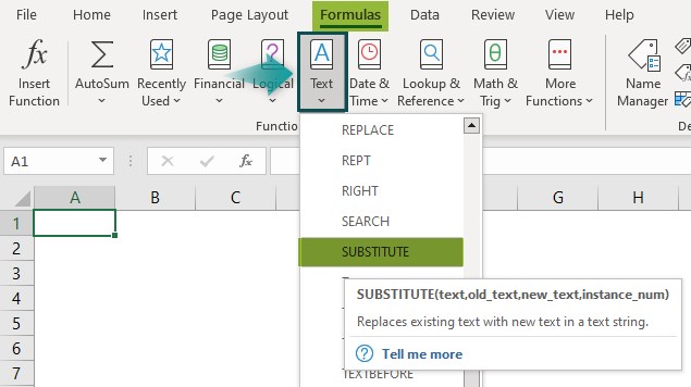
First, choose the cell for the output – select the “Formulas” tab – go to the “Function Library” group – click the “Text” drop-down – select the “SUBSTITUTE” function, as shown below.
The “Function Arguments” window opens. Enter the arguments as cell values or Excel cell references in their respective fields. Then, click “OK”, as shown below.

Method #2 – Enter in the worksheet manually
Ensure that our source text string is complete and accurate. Also, we should know what text and its instances we have to replace with the required new text in the specified text string.
- Select the target cell.
- Type =SUBSTITUTE( in the cell. [Alternatively, type =S or =SU and double-click the SUBSTITUTE function from the Excel suggestions.
- Enter the arguments as values or cell references.
- Close the brackets.
- Finally, press Enter to view the updated text string.
Basic Example
We will replace the required text to correct the book names using SUBSTITUTE function in Excel.
In the following table, the data is,
- Column A contains incorrect book names.
- Column B contains the Old_text to be replaced.
- Column C contains the New_text to replace the Old_text.
- Column B contains the Text Instance.
- Column E displays the corrected data.

The steps to correct the book names using SUBSTITUTE function in Excel are:
Step 1: Select cell E2, enter the formula =SUBSTITUTE(A2,B2,C2), and press the “Enter” key. The result is shown below.

[Alternatively, we can select the target cell E2 and click Formulas – Text – SUBSTITUTE to open the Function Arguments window.

Then, enter the three mandatory SUBSTITUTE() arguments in the Function Arguments window as cell references or values.

And once we click OK, the SUBSTITUTE() will get executed and updated text string.]
Step 2: Drag the formula from cell E2 to E7 using the fill handle. [Note: We will enter different formulas for the cells E8 and E9].

Step 3: Select cell E8, enter the formula =SUBSTITUTE(A8,B8,C8,D8), including the instance_num argument, and press the “Enter” key. The output is shown below.

Step 4: Select cell E9, enter the formula =SUBSTITUTE(“Reminders Of Hime”,”e”,””,3), and press the “Enter” key.

The complete output is shown above in column E. In cells E8 and E9, the requirement is to replace a specific instance of the old text in the given text string with a new text. So, the function needs all four arguments to return the required updated text string.
[Note: Ensure the specified texts’ cases are correct to avoid potential errors. Also, the text values should be in double quotations when directly supplying the values arguments to the function.]
Examples
We will understand the SUBSTITUTE function in Excel using advanced scenarios.
Example #1
We will use the SUBSTITUTE function in Excel when the given text string requires multiple substitutions.
In the following table, the data is,
- Column A shows a list of Engineering course abbreviations.
- Column B will display the full form of the courses.

The steps to get the full form of courses using the SUBSTITUTE function in Excel are:
Step 1: Select the target cell B2, enter the nested formula
=SUBSTITUTE(SUBSTITUTE(A2,”M”,”Mechanical”),”E”,”Engineering”), and press the “Enter” key. The result is shown below.

Step 2: Select the target cell B3, enter the nested formula
=SUBSTITUTE(SUBSTITUTE(A3,”R”,”Robotics”),”M”,”Mechatronics”), and press the “Enter” key. The result is shown below.

Step 3: Select the target cell B4, enter the nested formula =SUBSTITUTE(SUBSTITUTE(SUBSTITUTE(A4,”M”,”Materials”,1),”M”,”Mineral”,2),”E”,”Engineering”), and press the “Enter” key. The result is shown below.

[Output Observation: Depending on the number of substitutions required in a given text string at a time, the number of SUBSTITUTE functions in the nested formula will vary.
For instance, the text strings in rows 2 and 3 require the replacement of two text values. So, each nested formula in the target cells contains two SUBSTITUTE functions. On the other hand, the third text string (Refer to row 4) requires replacing three text values. And thus, the formula in the target cell B4 includes three SUBSTITUTE functions.]
Example #2
We will update the word count using the SUBSTITUTE function in Excel with TRIM(), and LEN() Excel function.
The following table shows a list of quotes by famous personalities.

The steps to find the word count using SUBSTITUTE(), TRIM() and LEN() functions are:
Step 1. Select cell B2, enter the formula =(LEN(TRIM(A2))-LEN(SUBSTITUTE(A2,” “,””)))+1, and press the “Enter” key. The result is shown below.

Step 2: Drag the formula from cell B2 to B6 using the fill handle.

The output is shown above.
[Output observation: Let us consider the formula in cell B6 to see how it works. First, the TRIM() removes unnecessary spaces at the start and end of the text string in cell A6. Then, the first LEN() calculates the text string length and returns a value of 57.
The SUBSTITUTE() removes the spaces from the text string in cell A6, and the second LEN() returns the text string length as 48. Finally, the formula determines the difference between the two calculated values, 57 and 48, which is the count of spaces in the text string. And it adds the value 1 to it to give the result as 10. The value 1 added to the difference is because a text string word count is ideally one more than the number of spaces.]
Example #3
We will use the SUBSTITUTE with VLOOKUP(), and LEFT() excel function to display the contact number of a particular student, Francis Vasquez, in a specific format.
The following table contains a list of student names and their contact numbers.

The procedure to apply the SUBSTITUTE(), VLOOKUP() and LEFT() functions are:
First, select the target cell E2, enter the formula
=SUBSTITUTE(SUBSTITUTE(VLOOKUP(D2,A1:B11,2,0),LEFT(VLOOKUP(D2,A1:B11,2,0),1),”(“&LEFT(VLOOKUP(D2,A1:B11,2,0),1)),”-“,”)”,1), and press the “Enter” key.

The output is shown above.
[Output Observation: There are two values to substitute in the contact number. The first is inserting an opening parenthesis before the first number in the phone number, and the second is replacing the first hyphen with a closing parenthesis.
So, first, the VLOOKUP() looks up the contact number in column B, corresponding to the name Francis Vasquez mentioned in cell D2, 608-202-9123. Then the LEFT() returns the first character in the phone number from the left, 6.
Next, the inner SUBSTITUTE() replaces the value 6 with ‘(6‘, and then the outer SUBSTITUTE() replaces the first hyphen in the phone number with ‘)‘. Thus, the formula returns the determined contact number in the required format as (608)202-9123.]
Important Things To Note
- The SUBSTITUTE function in Excel replaces a specific text in the given text string with another text if we omit the optional argument, instance_num.
- The function is case-sensitive. The supplied old_text case does not match the case of the text we need to replace in the given text string. Otherwise, the new_text case will be incorrect and not the accurate output.
- The SUBSTITUTE() does not support wildcard characters such as asterisks, question mark, etc.
- When directly supplying texts as arguments to the SUBSTITUTE(), ensure they are in double quotations. Otherwise, the function returns the #NAME? error.
Frequently Asked Questions (FAQs)
The SUBSTITUTE function in Excel is in the Formulas tab. Click Formulas > Text > SUBSTITUTE to access it.
We can use the SUBSTITUTE() in Excel to remove spaces as follows:
The below table shows two text strings and the requirements for removing spaces from them.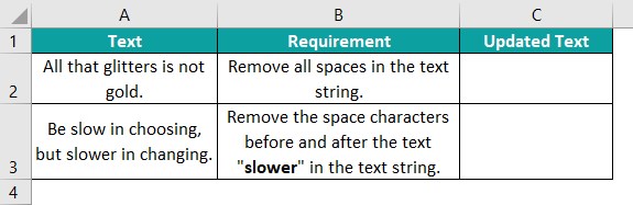
The steps to remove spaces are:
Step 1: Select cell C2, enter the formula =SUBSTITUTE(A2,” “,””), and press the “Enter” key.
[Note: The second argument is a space within double quotes, and the third argument is a double quote without space.]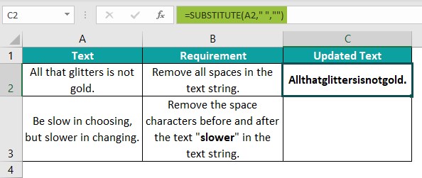
Step 2: Select cell C3, enter the formula =SUBSTITUTE(SUBSTITUTE(A3,” “,””,5),” “,””,5), and press the “Enter” key.
[Note: The requirement is to remove two space characters, one before and one after the text “slower”. Thus, we need to use multiple SUBSTITUTE functions.]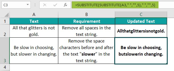
The output is shown above.
[Output observation for cell C3: First, the inner SUBSTITUTE() removes the space character at the 5th position in the source text string. Then, the space after the text “slower” becomes the 5th space character. So the outer SUBSTITUTE() removes it to return the text string.]
The SUBSTITUTE function might not work for the following reasons:
– The supplied old_text case differs from the text case in the given text string. Otherwise, the new_text case is incorrect.
– The text values inserted contain wildcard characters, which the function does not support.
– The text values directly inserted are not in double-quotes.
– We are trying to replace text in the required text string in a protected cell.
Use this SUBSTITUTE Function In Excel Template to follow along with the examples in this article.
Download Excel TemplateRecommended Articles
Continue with these related resources when you want the next practical step in this topic.
Explore the full Excel Text Functions guide or browse Excel Resources.