
What Is LARGE Function In Excel?
The LARGE function in Excel helps the user find the largest value, 2nd largest, 3rd largest, and so on…, in a given dataset or a selected cell range. Unlike MAX() or sorting in descending order to find the largest value, the function determines the kth-largest value w.r.t the value’s relative position.
The LARGE Excel function is an inbuilt Statistical function, which means that we can insert the formula from the “Function Library” or enter it directly in the worksheet. For example, the below table shows a list of heights and weights.

- To determine the second-highest height, select cell F2, enter the formula =LARGE(A2:A11,2), and press the “Enter” key.
- To determine the highest weight values, select cell F3, enter the formula =LARGE(B2:B11,1), and press the “Enter” key.

The above image shows the output in cells E2 and E3, using the LARGE Excel function.
Use this LARGE Excel Function Template to follow along with the examples in this article.
Download Excel TemplateKey Takeaways
- The LARGE Excel function calculates the kth-largest value in the specified array range, considering the data points in descending order. Thus, the function is useful for finding values, such as top scores and second and third-highest values in a given array.
- The LARGE() takes the arguments, array, and k, as input. The first argument is an array range reference. And the second argument can be a number or a cell reference to a number.
- The function LARGE(array,1) will return the largest value in the given array. And if the array has m values, the function LARGE(array,m) output will be the least value in the specified array.
- We can use the LARGE() with other Excel functions such as ROWS, INDEX, MATCH, and COUNTIF.
LARGE() Excel Formula
The LARGE Excel formula syntax is:

The arguments of the LARGE Excel formula are:
- array: The array or a cell range to calculate the kth-largest value. It is a mandatory argument.
- k: The position from the largest value in the dataset to return. It is a mandatory argument.
How To Use LARGE Excel function?
We can use the LARGE Excel function in 2 methods, namely,
- Access from the Excel ribbon.
- Enter in the worksheet manually.
#1 Method – Access from the Excel ribbon
First, choose a cell for the output – select the “Home” tab – go to the “Function Library” group – click the “More Functions…” drop-down – click the “Statistical” option right arrow – select the “LARGE” function, as shown below.

The “Function Arguments” window appears. Enter the “Array” and “K” arguments as cell values or cell references in Excel in their respective fields, and click “OK”, as shown below.

#2 Method – Enter in the worksheet manually
First, ensure the array range is accurate and error-free.
- Select the target cell,
- Type =LARGE( in the selected cell. [Alternatively, type =L and double-click the LARGE() function from the Excel suggestions.]
- Enter the arguments as values or cell references.
- Close the brackets.
- Press the “Enter” key.
#Basic Example
We will find the 5th– most expensive smartphone from the list using LARGE Excel function.
The table below shows smartphone models and their prices. [Column B data format is set to Currency.]

The procedure to apply the LARGE Excel function is:
Select cell B14, enter the formula =LARGE(B2:B11,5), and press the “Enter” key.

The output is shown above.
[Note: Since the B14 cell’s data format is Currency, the output is a currency value. Otherwise, if the Number Format were General, the function output would be a number.]
[Alternatively, select the target cell B14 and click Formulas – More Functions – Statistical – LARGE to open the Function Arguments window.

The “Function Arguments” window pops up. Enter the two argument values. Click “OK”.

[Output Observation: The LARGE() sorts the data points in the specified array range in descending order and then returns the required kth– largest value. So, in the above example, the sorted array values are {999, 840, 800, 700, 699, 699, 699, 599, 449, 429}. And hence the LARGE() returns the value of $699 as the 5th– highest price from the price list.]
Examples
We will learn some advanced scenarios using LARGE Excel function.
Example #1
We will use the LARGE Excel function along with the INDEX() and MATCH() Excel functions to determine the top 5 profitable companies from the given list of firms.
The first table below lists US companies and their 2021 annual profits in billions of dollars, and we will update the results in the second table.

The steps to use the LARGE Excel function with INDEX() and MATCH() are:
1: Select cell F3, enter the formula =INDEX($A$2:$A$11,MATCH(LARGE($B$2:$B$11,E3),$B$2:$B$11,0)), and press the “Enter” key.

2: Drag the formula from cell F3 to F7 using the fill handle.

The output is shown above.
Output Observation: Consider the formula in the target cell F7. The LARGE() takes the array range $B$2:$B$11 as the array argument and the cell reference to the value 5, E7, as the k argument. So, it sorts the annual profit values in descending order to return the 5th– largest profit value, $48.3 billion.
Then, the MATCH() checks for the position of the profit value of $48.3 billion in the array range $B$2:$B$11. And it returns a value of 8, as $48.3 billion is the 8th value in the specified array. Finally, the INDEX() returns the value at the 8th position in the array range $A$2:$A$11, JP Morgan Chase.
Thus, the above example shows that the LARGE() can determine the top N values using absolute cell reference to the given array and k values, varying from 1 to N. And the entire formula relies on the LARGE() return value to get the required results in the target cells.]
Example #2
We will use the LARGE and ROWS() Excel function to show how the function can help sort an array range quickly in descending order.
In the following table, column A contains a list of single-family house sizes in square feet.

The steps to sort the size values in descending order using LARGE() and ROWS() functions are.
1: Select cell C2, enter the formula =LARGE($A$2:$A$16,ROWS(A$2:A2)), and press the “Enter” key.

2: Drag the formula from cell C2 to C16 using the fill handle.

The output is shown above.
[Output Observation: In the above example, the ROWS() returns the count of rows in the specified reference in each target cell. Then, the LARGE function takes the ROWS() output as the k argument value and returns the kth-largest value in the target cell.
For instance, the ROWS() in cell C2 returns the value of 1. And then, the LARGE() returns the largest size value from the data points in column A, 2590. Likewise, the ROWS() in cell C16 returns the count of rows as 15. So, the LARGE() returns the 15th-largest house size, 1900.
Thus, in this way, the LARGE() sorts the given list of values in descending order.]
Example #3
The LARGE and COUNTIF() Excel function work well for date and time values.
Let us assume today’s date is 10-08-2022 and determine the date of the next meeting.
The following table contains a list of meeting schedules.

The steps to use the LARGE Excel function with COUNTIF() are:
1: Select cell B11, enter the formula =LARGE($B$2:$B$7,COUNTIF($B$2:$B$7,”>”&B9)), and press the “Enter” key.

2: We get the output ‘44784’, as shown below. Select cell B11 and set the Number Format in the Home tab as Short Date to get the result in the proper date format.

Once we set the required date format, the output will be ‘11-08-2022’, as shown below.

[Output Observation: The COUNTIF() counts the dates in the cell range B2:B7 greater than today’s date. As all the values are future dates, it returns a value of 6. Then the LARGE() returns the 6th-largest date from the list, 11-08-2022.
[Note: The LARGE() considers the farthest date as the largest value in an array of dates.]
Important Things To Note
- The LARGE Excel function ignores non-numeric data, such as text, logical values, and empty cells.
- If the array range provided as the first argument contains error values, the LARGE function return value will be an error.
- LARGE Excel function return value will be a #NUM! error,
- If the selected array or the cell range is empty.
- If the kth value is less than or equal to 0, or more than the number of values in the provided array.
Frequently Asked Questions (FAQs)
The LARGE function in Excel is in the Formulas tab. Click Formulas – More Functions – Statistical – LARGE to access it.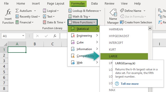
We can use the LARGE Excel function with VLOOKUP to find the year’s top performer.
The following table shows the maximum monthly sales achieved by a top performer each month.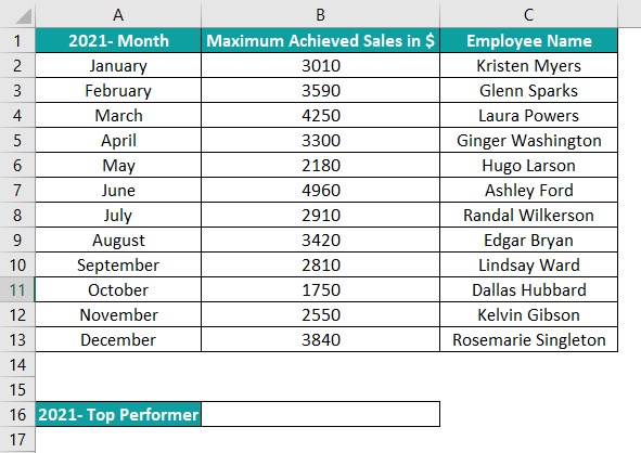
The procedure to find the year’s top performer using the LARGE Excel function with VLOOKUP are:
Select cell B16, enter the formula =VLOOKUP(LARGE(B2:B13,1),B2:C13,2,0), and press the “Enter” key.
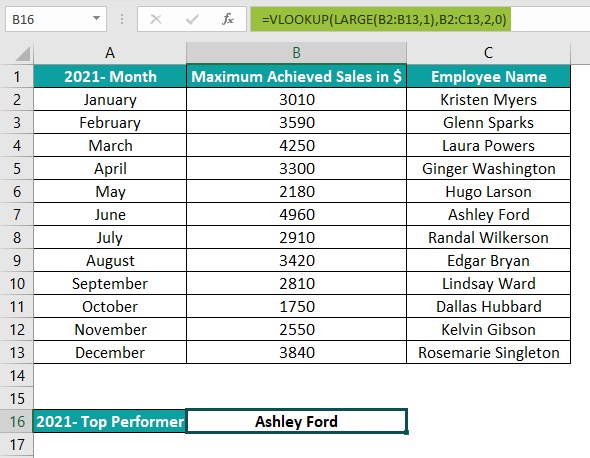
The output is 4960, as shown above, i.e., the highest sales value, and the VLOOKUP() looks up the employee name corresponding to the value and returns Ashley Ford.
A few reasons why the LARGE function might not work are:
– We provided an empty array, or the supplied array does not contain any numeric value.
– The argument k is a negative value.
– We entered a k value greater than the number of data points in the specified array.
Use this LARGE Excel Function Template to follow along with the examples in this article.
Download Excel Template