RANK Function In Excel

What Is RANK Function In Excel?

The RANK function in Excel is an inbuilt Statistical function that returns the rank of a numeric value in a given array of numbers. The rank gets assigned to a specific data point based on its size relative to the other values on the list.

Users can apply the RANK() to rank numbers in ascending or descending order.

For example, column A in the below table shows height in cm.

Suppose we have to rank the heights and display the rank order in column B. Then, the RANK function in Excel return value will give us the required result.

Once we execute the RANK() in cell B2 and drag the fill handle to copy the formula in cell range B3:B10, all the height values get ranked.

The RANK function return value in the above illustration shows the ranks in the descending order of height, the default order.

What Is RANK Function In Excel?

The RANK function in Excel returns the rank of a numeric value in an array of numbers relative to other numbers on the list.
The RANK formula in Excel is =RANK(number,ref,[order])
The RANK function in Excel ignores non-numeric values in the ref argument.
It assigns the same rank to duplicate data points.
The function takes two mandatory arguments, number, and ref. On the other hand, the third argument, order, is optional.
The third argument, order, has to be a non-zero number to ensure the RANK() returns the ranks in the ascending order.

RANK() Excel Formula

The RANK formula in Excel is:

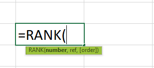
where,

number: The numeric value for which we need to determine the rank.
ref: The array of numeric values or reference to the array of numeric values.
order: A number that specifies how to rank the numeric values. If the order is 0, the ranking of numbers will be in descending order. And the RANK function in Excel without the order argument will also rank the values in descending order. On the other hand, a non-zero order value indicates an ascending order of ranking the numbers.

While the first two arguments in the RANK formula in Excel are mandatory, the argument order is optional.

Please Note: While the RANK function in Excel ignores non-numeric values in the ref argument, it assigns the same rank to duplicate data points.

Excel VBA – All in One Courses Bundle (35+ Hours of Video Tutorials)

If you want to learn Excel and VBA professionally, then Excel VBA All in One Courses Bundle (35+ hours) is the perfect solution. Whether you’re a beginner or an experienced user, this bundle covers it all – from Basic Excel to Advanced Excel, Macros, Power Query, and VBA.

Start Learning Now

How To Use RANK Excel Function?

The steps to use the RANK function in Excel are:

First, ensure the source data, containing numbers, is complete and without empty cells. Otherwise, we will get the #N/A error.
Select the target cell, enter the RANK() with the mandatory and required optional arguments, and press Enter.
Drag the fill handle downwards to copy the RANK() in the required cell range.

Here is a RANK function in Excel example to understand the above steps:

Consider the below table showing the students’ scores in Science.

Suppose we need to rank the students based on their Science scores. Here is how we can get the required result using RANK function in Excel.

Step 1: Select cell C2, type the required RANK(), and press Enter.

=RANK(B2,$B$2:$B$11)

Alternatively, we can select cell C2 and choose the option Formulas > More Functions > Compatibility > RANK to open the Function Arguments window.

In the Function Arguments window, we can enter the argument values and click OK to get the RANK() output.

Step 2: Drag the fill handle downwards to copy the RANK() in the cell range C3:C11.

In the above RANK function in Excel example, the ranking is in descending order, which is the default, as the formula does not contain the third argument, order. While the student with the highest science score ranks first, the one with the lowest score gets the last rank, 10. These positions are relative to the other students’ scores on the list.

Examples

Here are a few scenarios where we can use the RANK function in Excel.

Example 1

Let us see how the RANK function in Excel returns the ranks in ascending order.

Consider the below list of runners and their race completion timings.

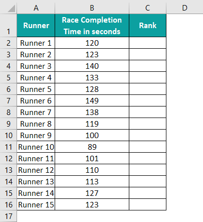
Here is how we can use the RANK function in Excel to rank them. The ranking has to be in ascending order, as the runner who takes the least time to finish the race should rank on top.

Step 1: Select cell C2, type the required RANK(), and press Enter.

=RANK(B2,$B$2:$B$16,1)

Step 2: Drag the fill handle downwards to copy the RANK() formula in the range C3:C16.

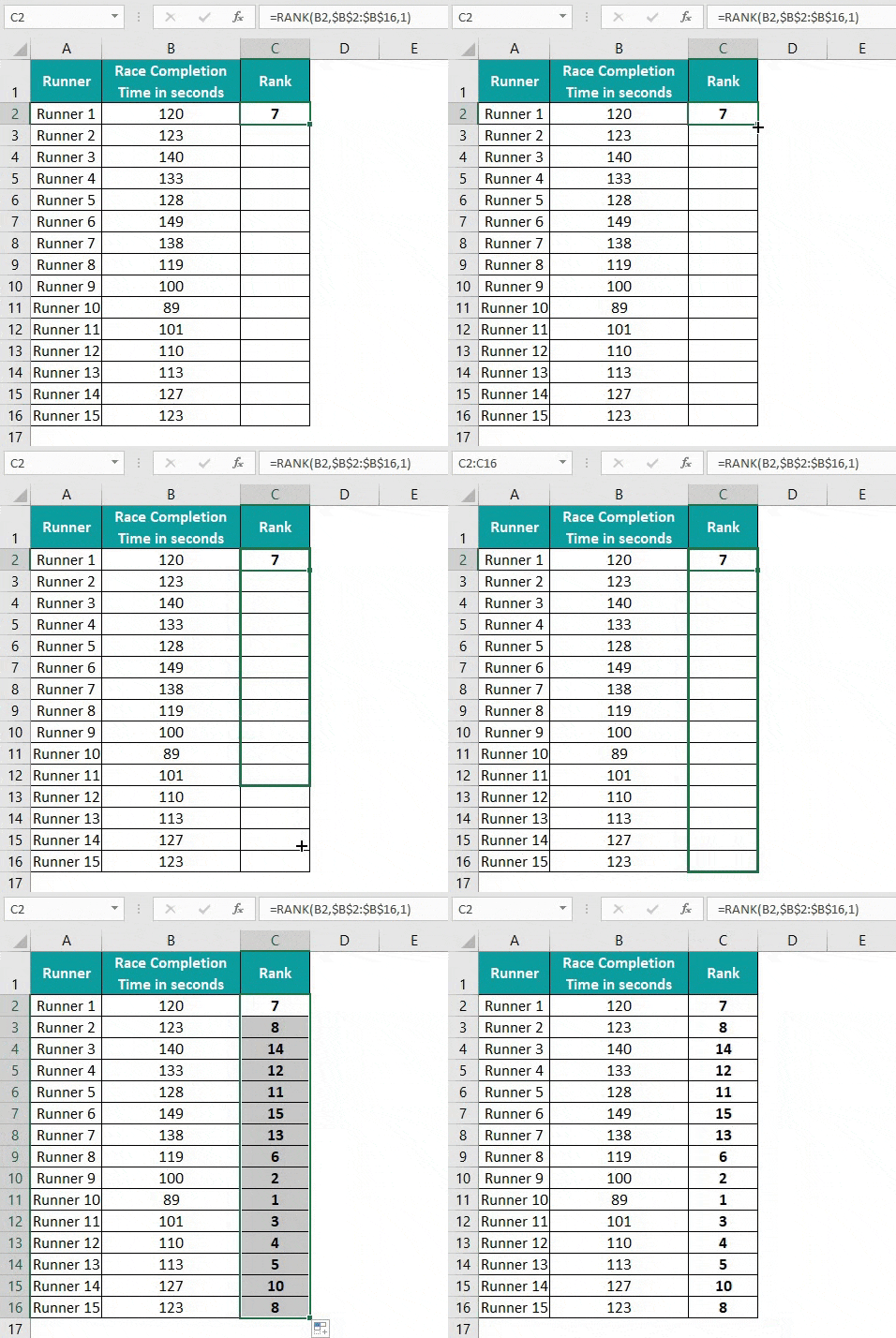
Runner 10 took the least time to finish the race, 89 seconds. Thus, the RANK() ranks Runner 10 as rank 1.

Please Note: Runners 2 and 15 take the same time to complete the race, 123 seconds. So, both get the same rank, 8, relative to other runners’ timings. And the rank list skips the 9^th position and displays the rest of the ranks, till 15.

Example 2

Here is an example of the RANK function in Excel without duplicates.

The below table shows the employees’ task completion details.

If we use the RANK function in Excel, each employee set EMP_101 and EMP_110, EMP_102 and EMP_107, and EMP_104 and EMP_108 would be at the same ranks.

However, we can use the RANK function in Excel without duplicates in the result, thus breaking the ties.

Step 1: Select cell C2, enter the below formula containing the RANK() and COUNTIF(), and press Enter.

=RANK(B2,$B$2:$B$11)+COUNTIF($B$2:B2,B2)-1

Step 2: Drag the fill handle downwards to copy the formula in the cell range C3:C11.

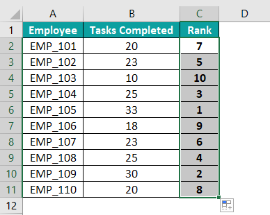
While the RANK function in Excel calculates the rank as explained previously, the COUNTIF() returns a value of 2 for the second occurrence of the same value in column B. So the term -1 ensures the final sum in each cell is unique, thus resulting in ranks without duplicates.

Example 3

Though the RANK function in Excel is a Statistical function, we will find it in the Compatibility functions group. The reason is that Excel offers new functions RANK.AVG and RANK.EQ, from Excel version 2010 and above, provides more accurate results.

Please Note: The arguments for RANK.AVG() and RANK.EQ() are the same as those we supply to RANK().

Consider the below sales data table.

This example shows the results when using the RANK function in Excel, RANK.AVG and RANK.EQ to rank the sales offices based on their sales results.

Here is how we can use the three RANK functions and update columns C, D, and E.

Step 1: Select cell C2, type the RANK() mentioned in the Formula Bar in the below image, and press Enter.

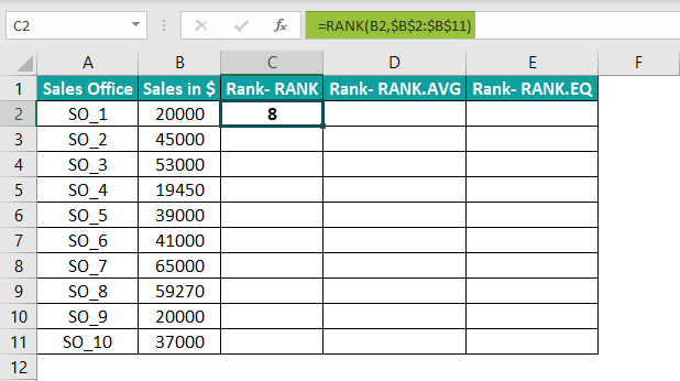
Step 2: Drag the fill handle downwards to copy the formula in the range C3:C11.

Step 3: Select cell D2, and type the RANK.AVG() mentioned in the Formula Bar as shown in the image below, and press Enter.

Step 4: Drag the fill handle downwards to copy the formula in the cell range D3:D11.

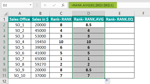
Step 5: Select cell E2, and type the RANK.EQ() mentioned in the Formula Bar in the image below, and press Enter.

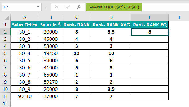
Step 6: Drag the fill handle downwards to copy the formula in cell range E3:E11.

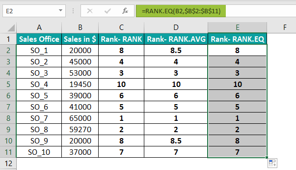
The RANK() and RANK.EQ() treat the values occurring multiple times in the value range in the same manner. On the other hand, the RANK.AVG() assigns an average rank to such values. For example, the function assigns a rank of 8.5 to the sales value of $20,000, as it appears twice in the data range.

Important Things To Note

The RANK function in Excel does not apply to text data or a text representation of numbers.
By default, the function orders the ranking numbers in descending order.
The RANK() assigns the same rank to a value appearing multiple times in the value range.
EQ() and RANK.AVG() are the improved versions of the RANK(), providing more accurate results.
The RANK(), when used with other Excel functions, such as COUNTIF, yields fruitful results.
We must ensure the source data is complete and has no any empty cells to avoid #N/A

Frequently Asked Questions

Where is the RANK function in Excel?

The RANK function in Excel is available in the Formulas Tab. Click on Formulas > More Functions > Compatibility > RANK.

On the other hand, we can find the newer functions RANK.AVG and RANK.EQ, in the Statistical functions category.

FAQ 1.1

How do you rank highest to lowest in Excel?

We can rank the highest to lowest in Excel using the RANK(). And for that, we need to set its third argument (order) as 0. Otherwise, we can apply the RANK() without the third argument to rank the number range in the highest to lowest order.

How to use RANK function in excel with multiple conditions?

We can use RANK function in Excel with multiple conditions by applying the below steps.

Let us see the process with an example.

The below table shows students’ scores in one subject and their overall aggregates.

Suppose we need to rank them based on their marks in Subject 1 and use the overall aggregate to break any ties. The steps are:

Step 1: Select cell D2 and type the formula containing the RANK and COUNTIFS functions mentioned in the Formula Bar in the below image. And then press Enter.

FAQ 2.1

Step 2: Drag the fill handle downwards to copy the formula in the cell range D3:D6.

In the above example, students Gwendolyn Fleming and Eula James have the same score in Subject 1. Therefore, the RANK() would assign the same rank, 4, to both students, based on the first criterion of score position relative to the other students’ scores in the list.

But the second criterion, the overall aggregate, introduced by the COUNTIFS(), will help rank them uniquely, as depicted in the above image. Thus, in this way, we can use the RANK() to rank values based on multiple criteria.

Download Template

This article must be helpful to understand the RANK Function in Excel, with its formula and examples. You can download the template here to use it instantly.

RANK Function In Excel Download

RANK Function In Excel