
What Is AGGREGATE Excel Function?
The AGGREGATE Excel function returns the result of the specified aggregate operation performed on columns of data or the vertical range. Users can apply Excel functions such as SUM, AVERAGE, MAX, and COUNT, using the AGGREGATE() function. It also provides the choice to ignore error values and hidden rows.
The AGGREGATE function in Excel is an inbuilt function which means we can enter the formula directly in the worksheet or insert it from the “Math & Trig” option from the “Function Library”.
Use this AGGREGATE Excel Function Template to follow along with the examples in this article.
Download Excel TemplateFor example, the first table below shows a student’s scores in eight subjects.
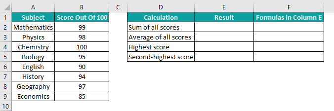
To update the results of the required calculations listed in the second table, enter the AGGREGATE() formulas =AGGREGATE(9,4,B2:B9), =AGGREGATE(1,4,B2:B9), =AGGREGATE(4,4,B2:B9), and =AGGREGATE(14,4,B2:B9,2) in the cells E2, E3, E4, and E5, respectively.
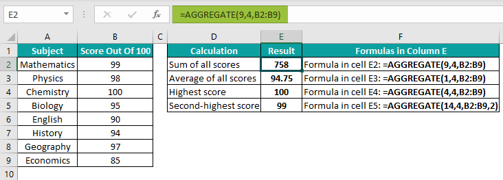
The output is shown above. The AGGREGATE Excel function in each target cell differs according to the specified aggregate operation, such as SUM and AVERAGE in cells D2 and D3, respectively.
Key Takeaways
- The AGGREGATE Excel function helps apply aggregate operations, such as SUM and AVERAGE, on columns of data or a vertical range. However, we cannot use the function for the row values or a horizontal cell range.
- The functions give a choice to skip hidden rows and error values while executing the specific aggregate operation, thus overcoming the limitations of conditional formatting.
- The AGGREGATE() has two syntax formats, array and reference.
- Functions such as LARGE, SMALL, PERCENTILE, and QUARTILE require the additional argument k.
AGGREGATE() Excel Formula
The AGGREGATE Excel formula has two syntaxes, namely,
- Array Format.
- Reference Format
#Syntax 1 – The Array Format syntax of the AGGREGATE Excel formula is:
The Array Format arguments of the AGGREGATE Excel formula are:
- function_num: A number that refers to the aggregate operation we want to perform. It can be from 1 to 19. It is a mandatory argument.
| function_num | Function |
|---|---|
| 1 | AVERAGE |
| 2 | COUNT |
| 3 | COUNTA |
| 4 | MAX |
| 5 | MIN |
| 6 | PRODUCT |
| 7 | STDEV.S |
| 8 | STDEV.P |
| 9 | SUM |
| 10 | VAR.S |
| 11 | VAR.P |
| 12 | MEDIAN |
| 13 | MODE.SNGL |
| 14 | LARGE |
| 15 | SMALL |
| 16 | PERCENTILE.INC |
| 17 | QUARTILE.INC |
| 18 | PERCENTILE.EXC |
| 19 | QUARTILE.EXC |
- options: A number that indicates which values we require the AGGREGATE Excel function to skip in the dataset while executing the calculations. It can be from 0 to 7. It is a mandatory argument.
| Options | Values- Ignored |
|---|---|
| 0 (or omitted) | Ignore nested SUBTOTAL and AGGREGATE functions |
| 1 | Ignore hidden rows, nested SUBTOTAL, and AGGREGATE functions |
| 2 | Ignore error values, nested SUBTOTAL and AGGREGATE functions |
| 3 | Ignore hidden rows, error values, nested SUBTOTAL, and AGGREGATE functions |
| 4 | Ignore nothing |
| 5 | Ignore hidden rows |
| 6 | Ignore error values |
| 7 | Ignore hidden rows and error values |
- array: The reference to an array of values on which we require to apply the AGGREGATE(). It is a mandatory argument.
- k: An integer representing the required data’s position in the array. Typically, functions such as LARGE, SMALL, PERCENTILE, and QUARTILE require this additional argument. It is an optional argument.
| Function | k- Interpretation |
|---|---|
| LARGE | Return the kth largest value |
| SMALL | Return the kth smallest value |
| PERCENTILE.INC | Return the kth percentile value |
| PERCENTILE.EXC | Return the kth percentile value |
| QUARTILE.INC | Return the kth quartile value |
| QUARTILE.EXC | Return the kth quartile value |
#Syntax 2 – The Reference Format syntax of the AGGREGATE Excel formula is:

The Reference Format arguments of the AGGREGATE Excel formula are:
- function_num and options have the same interpretation as explained in the Array Format.
- ref1, …: The numeric values on which we require to apply the aggregation function. And the function can accept 2 to 253 ref arguments.
The argument’s function_num, options, ref1, and ref2 are mandatory in this syntax format. And the following numeric values after ref2 are optional.
Below are a few critical facets of the AGGREGATE Excel function we should consider while using the function:
- If the aggregate operation we want to perform requires the ref2 value and we do not supply it to the AGGREGATE(), the function will return the #VALUE!
- Suppose we provide 3-D references as ref arguments to the AGGREGATE(), then the function will return the #VALUE!
- The AGGREGATE() function does not work for horizontal ranges of values.
How To Use AGGREGATE Excel Function?
We can use the AGGREGATE Excel function in 2 methods, namely,
- Access from the Excel Ribbon.
- Enter in the worksheet manually.
#Method 1 – Access from the Excel Ribbon
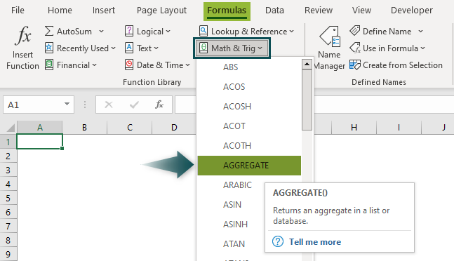
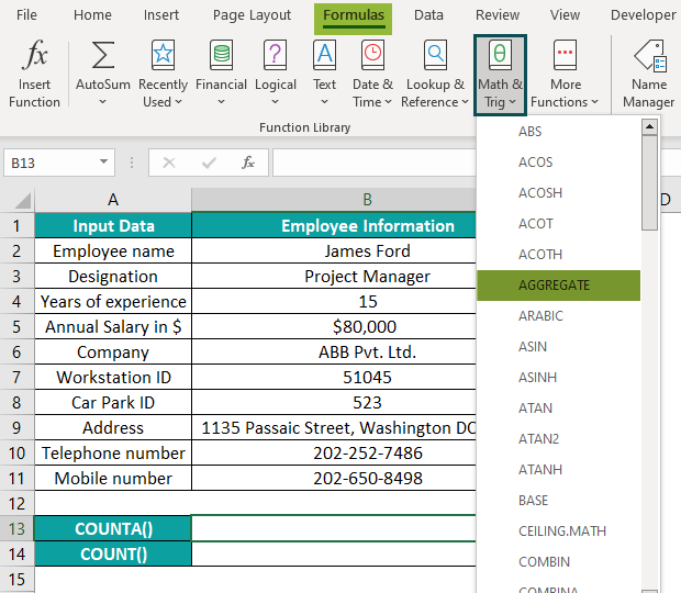
First, choose the target output cell → select the “Formulas” tab → go to the “Function Library” group → click the “Math & Trig” drop-down → select the “AGGREGATE” function, as shown below.
The “Select Arguments” window pops up.
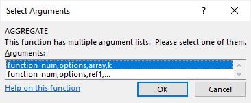
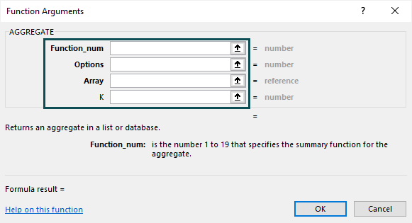
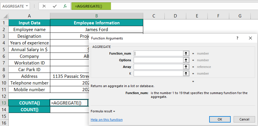
- If we choose the Array Format and click “OK”, the “Function Arguments” window opens with the “Array Format” argument fields, as shown below. Enter the arguments accordingly and click “OK”.
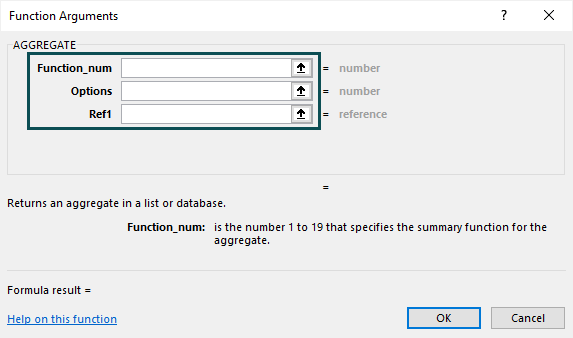
- If we choose the Reference Format and click “OK”, the “Function Arguments” window opens with the “Reference Format” argument fields, as shown below. Enter the arguments accordingly and click “OK”.
#Method 2 – Enter in the worksheet manually
- First, ensure our source data is complete and in vertical ranges.
- Next, select the target cell for the output.
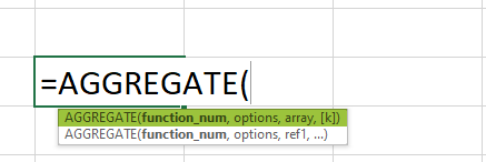
- Type the formula =AGGREGATE(. [Alternatively, type =A and double-click the AGGREGATE Function from the list of suggestions from Excel].
- Press the “Enter” key. We will get two syntaxes to select.
- Select the “Array Format or Reference Format” accordingly.
- Finally, press the “Enter” key.
#Basic Example
We will find the number of cells containing the employee’s information and the number of cells containing numbers using AGGREGATE Excel function.
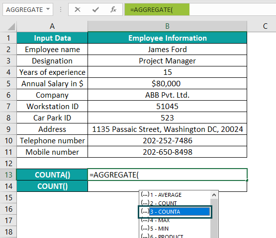
The below table contains an employee’s information.
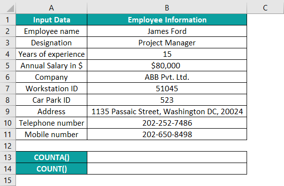
The steps to get employee details using AGGREGATE Excel function are:
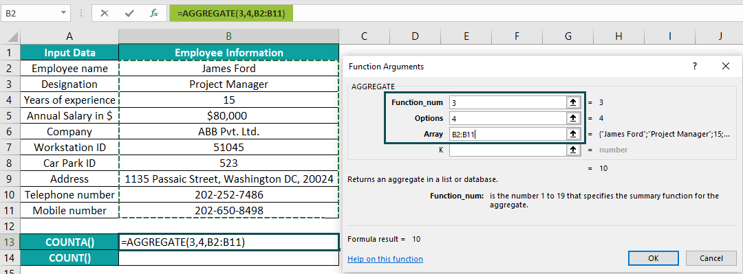
- Select cell B13, enter the formula =AGGREGATE(, choose 3 [COUNTA] in the drop-down list that appears, as shown below. The formula so far is =AGGREGATE(3

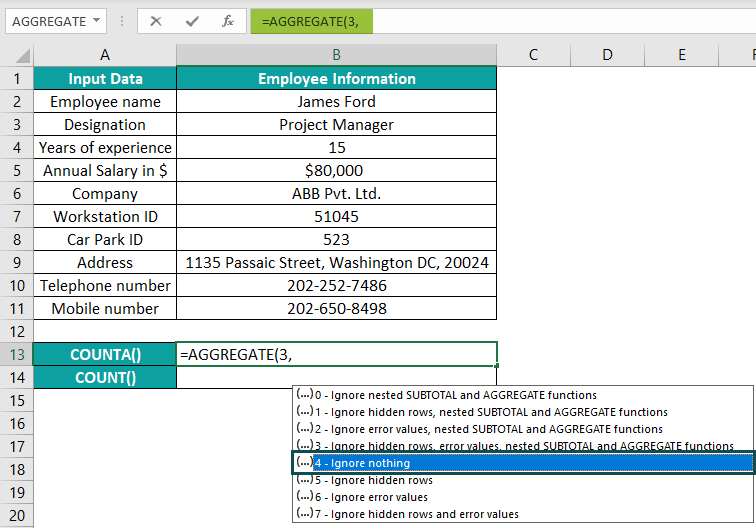
- In continuation with the formula, enter a ‘,’ after which we will see a drop-down list to select the options argument. In this case, we shall double-click on option 4 (Ignore nothing). The formula now is =AGGREGATE(3,4

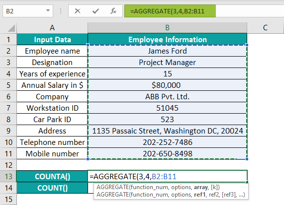
- In continuation with the formula, enter a ‘,’, choose the array range i.e., B2:B11, and close the brackets. The complete formula is =AGGREGATE(3,4,B2:B11).

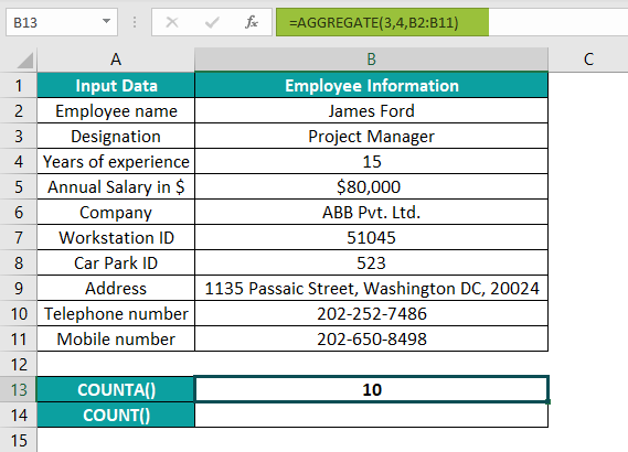
- Finally, press the “Enter” key. The output is 10, as shown below.

[Alternatively, select cell B13 and click Formulas → Math & Trig → AGGREGATE to open the Function Arguments window.
The below dialog box will pop up. Then, choose the Array format of the AGGREGATE() syntax. Then, press OK to open the Function Arguments window.

Enter the AGGREGATE() arguments in the Function Arguments window as cell values or cell references.
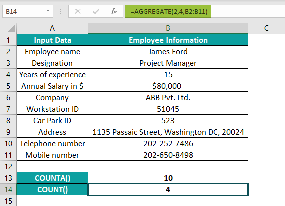
And once we click OK, the COUNTA() output will appear in the target cell B13.] - Next, to determine the number of cells containing numbers in the cell range B2:B11, select cell B14, enter the formula =AGGREGATE(2,4,B2:B11), and press the “Enter” key. [Note: Double-click on 2 to choose the COUNT().]
The output is 4, as shown above, as cells B4, B5, B7, and B8 contain numbers.
The output is 4, as shown above, as cells B4, B5, B7, and B8 contain numbers.
Examples
We will understand some advanced scenarios using the AGGREGATE Excel function examples.
Example #1
We will use the reference format of AGGREGATE Excel function syntax to determine the median annual salary from the listed salaries.
The following table shows the salaries of fifteen employees.

The procedure to apply the AGGREGATE Excel function is:
First, select cell B18, enter the formula, using the reference format of syntax, =AGGREGATE(12,4,B2,B3,B4,B5,B6,B7,B8,B9,B10,B11,B12,B13,B14,B15,B16), and press the “Enter” key.

The output is 75800, as shown above.
[Special Note: Refer to steps 1, and 2 explained in the previous section to update the function_num and options arguments in the AGGREGATE().
The function will align the 15 values in numeric order. And as the dataset has an odd number of data points, the function returns the middle number as the median annual salary.
Alternatively, we can use the array format of the AGGREGATE() syntax to get the same result:
=AGGREGATE(12,4,B2:B16)
We might find applying the MEDIAN() more convenient. But the AGGREGATE() gives the desired results even when our dataset might have errors, hidden rows, or nested SUBTOTAL() and AGGREGATE().]
Example #2
We will use the AGGREGATE Excel function when the dataset contains error values and hidden rows.
The following table contains a list of prime numbers or factors.

To determine the product of the prime numbers, if we apply the PRODUCT() in the target cell B12, the output will be an error value, as cell B5 contains an error value.

The procedure to apply the AGGREGATE Excel function to get the required result despite an error value is:
First, select cell B12, enter the formula =AGGREGATE(6,6,B2:B11), and press the “Enter” key.

The function_num argument is 6 (PRODUCT), and the options argument is 6 (Ignore error values). Thus the AGGREGATE() ignores the error value in cell B5 and returns the product of the remaining data points.
Another scenario is if we hide row 7 and the error value in cell B5. And we do not want to include the hidden cell B7 value in the product.

So, now the formula will be: =AGGREGATE(6,7,B2:B11)

Here the argument options value is 7 (Ignore hidden rows and error values). Thus, the AGGREGATE() does not consider the hidden value (cell B7) and error value (cell B5) while calculating the multiplication product of the prime factors.
Thus, we can use the argument options to decide the values we want to ignore while applying the specific aggregate operation.
Example #3
The AGGREGATE Excel function can help us process arrays for specific operations without using Ctrl + Shift + Enter. For Example, we will find the maximum quantity ordered for a particular fruit.
The following table shows a list of fruits and their order details.

If we use the LARGE() function, it will involve array ranges. To execute it as an array formula, press Ctrl + Shift + Enter instead of the Enter key. Moreover, one of the ordered quantities for Banana is an error value (cell C19), so the LARGE() will return an error, as shown below.

Instead, the steps to apply the AGGREGATE Excel function to get the required result are:
Step 1: Select cell G2, enter the formula =AGGREGATE(14,6,C2:C21*(A2:A21=F2),1), and press the “Enter” key. The output is 650, as shown below.

The above function has function_num 14, which denotes the LARGE(). And the options argument is 6, which indicates Ignore error values.
On the other hand, the term (A2:A21=F2) returns TRUE for cells in column A containing the item Banana and FALSE for other cells in column A. The term C2:C21 lists the quantities in column C. And the term, C2:C21*(A2:A21=F2), lists the quantities cell-wise, showing the values corresponding to Banana and 0 for other items. And as we require the largest quantity, the k value is 1.
Finally, the AGGREGATE() determines the largest number from the quantity list, 650, while ignoring the error value.
Important Things To Note
- The AGGREGATE() argument, function_num, can take a value from 1 to 19. And the argument, options, can take a value from 0 to 7. Any values entered apart from these make the function return the #VALUE! error.
- The function output will be the #VALUE! error, if the aggregate operation we select requires the ref2 value and we do not provide it.
- We will also get a #VALUE! Error if the ref arguments in the AGGREGATE() are 3-D references.
Frequently Asked Questions (FAQs)
We can use the SUM AGGREGATE Excel function to determine the total units ordered.
The following table shows our source data, a list of gadgets, and ordered units with few error values.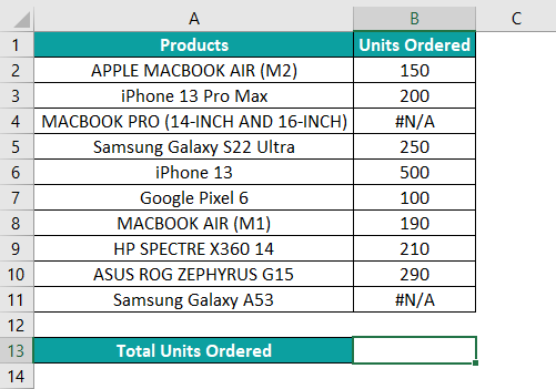
The steps to apply the SUM AGGREGATE function are:
Step 1: Select cell B13 and enter as indicated. First, enter =AGGREGATE(, double-click number 9 (SUM).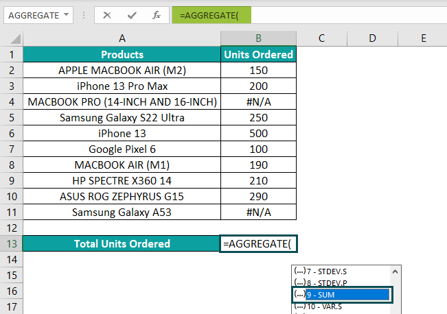
Step 2: Then enter a ‘,’ and double-click 6 (Ignore error values) to enter the options argument.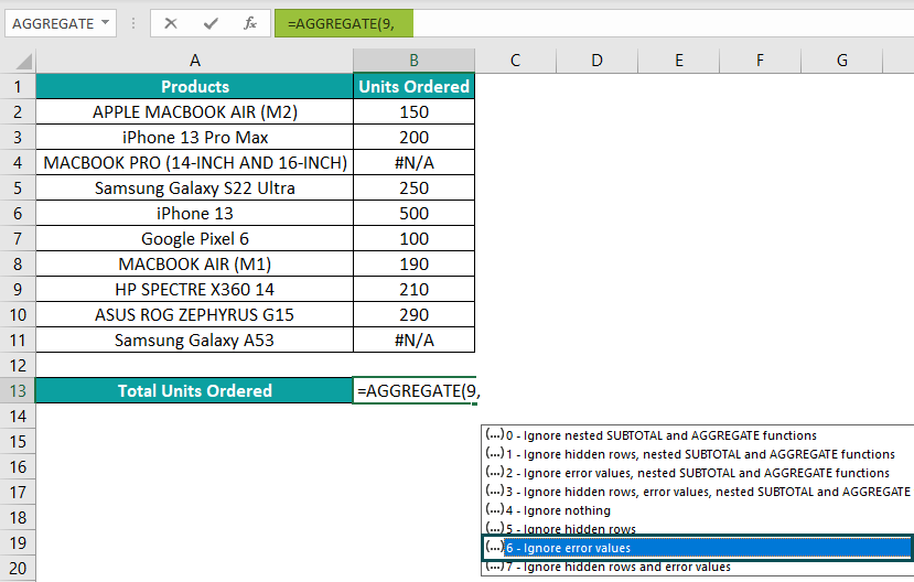
Step 3: Then enter a ‘,’ and select the array range to add the data points. Close the brackets.
The complete formula is =AGGREGATE(9,6,B2:B11).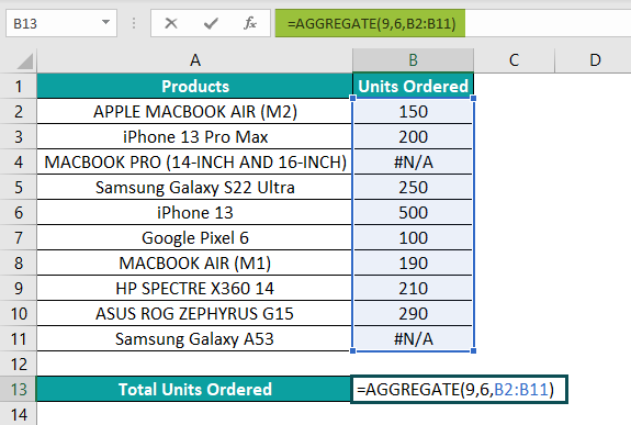
Step 4: Press the “Enter” key.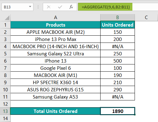
The output is 1890, as shown above i.e., the sum value, ignoring the error values.
The AGGREGATE Excel function ignores:
1. Hidden rows.
2. Error-values.
3. Nested SUBTOTAL() and AGGREGATE().
We can use the AGGREGATE Excel function to execute a specific aggregate operation, such as SUM or MEDIAN, for a data column or a vertical range.
Use this AGGREGATE Excel Function Template to follow along with the examples in this article.
Download Excel Template