
AutoSum Excel Definition
The AutoSum in Excel automatically adds the numeric values present in a range of cells. As a result, it saves time for users who would otherwise have to do the sum manually and risk making mistakes.
If you add numeric values in a column, the result gets displayed in a cell immediately below the range of cells. And for numeric values in a row, the total appears on the right of the cell range. For example, the image below shows an office inventory list, from cells B2 to B5. We can use the AutoSum function in the Formulas tab to add the quantity of items and display the result in cell B6.
Use this AutoSum In Excel Template to follow along with the examples in this article.
Download Excel Template
=SUM(B2:B5)

The Quantity range gets selected automatically, and the output comes as ‘63’.

Key Takeaways
- The AutoSum in Excel enables users to automatically calculate the sum of the values present in a particular column or a row. The result gets displayed in a cell immediately below the column cell range and to the right of the row cell range.
- It is accessible under the Home and Formulas options on the Excel menu.
- The shortcut to using the AutoSum formula is – ALT + =.
- This function can be used with other functions like Average, Count Numbers, Max, and Min, or to sum numeric values in multiple rows or columns values from the visible cells only using the Filter option.
AutoSum Excel Shortcut
Using AutoSum in Excel allows users to apply the SUM function in a cell faster. All you need to do is click on two keys: ALT and =.
The following steps will guide you to use the AutoSum in Excel shortcut:
Step 1: Press ALT with = sign in the cell below the range of cells in a column. You do not need to select the range of values manually.
Step 2: The SUM formula will appear in the specific cell with the range of cells containing numeric values to add. In the table from the previous illustration, the cell range would be B2 to B5, and thus the formula in cell B6 becomes:
=SUM(B2:B5)
How To Use AutoSum In Excel?
You may use the AutoSum formula in Excel in the following ways:
#1 – Using Excel Menu
You can find the AutoSum function in two different tabs on the Excel menu. One is under the Editing option in the Home tab, as shown below:

And the other way is through the AutoSum option present under the Function Library section of the Formulas tab:

In both scenarios, using the AutoSum function remains the same.
You may follow the below steps when applying the AutoSum formula from the Formulas tab.
- Select the cell where you aim to display the output.
- Click on the AutoSum icon in the Home tab or the “Formulas” tab on the Excel menu.
- Click on the “AutoSum” option next to the Insert Function.
- Automatically the SUM function appears in the cell chosen.
- You will see the reference of the range of cells with the values you wish to add. It acts as the arguments the SUM function requires to give the result.
- Click the Enter key
You can now see the total value in the specific cell.
#2 – Using Autosum Shortcut
- Choose the cell for displaying the output.
- While holding the ALT key, press the = key. It will enter the SUM excel function in the specific cell referencing the range of cells with the values you wish to add.
- Press the Enter key to get the output.
Here is a straightforward example to provide you with more clarity. The following image shows a table of marks obtained by a student in a competitive exam.
The aim is to add the scores of a sixth-grade student from different subjects present in the range of cells A2:E2 in cell F2. However, cell A2 has an alphabetical value.
While using AutoSum in Excel, you will observe that the function does not consider non-numeric values and processes positive and negative numeric values, like the SUM function.

The steps to add the given numbers are as follows:
Step 1: Select cell F2, where you wish to display the total marks.
Step 2: Click on the AutoSum function in the Formulas tab. The SUM function with the range B2:E2 will automatically appear in cell F2.
=SUM(B2:E2)

Step 3: Press Enter. The AutoSum in Excel will return the sum of marks in the range of cells B2:E2 and display the result 105 in cell F2.

Please note that the AutoSum formula in Excel considers only the numeric values in a given range of cells. The function did not consider cell A2 in the above example, as it holds an alphabetical value.
Examples
Here are some AutoSum in Excel examples to help you understand the function more comprehensively.
Example #1
You saw scenarios where a column or a row has numeric values, and the AutoSum function adds the values automatically when applied. You also saw how the formula behaves when a cell value is alphabetical.
Here you will see what happens if there is a blank cell in the range of the column or row in question.
The following image shows a table listing grocery items and their respective quantities.

- Column A shows Grocery Items
- Column B shows the Number of Packets
- Column C lists the Price in $ for each commodity
The steps to find the total number of packets and the total cost are as follows:
Step 1: First, select cell B8. Here is where you will see the total number of packets. Then, click on the AutoSum option from the Home or Formulas tab.

The range gets selected automatically from B5 to B7 instead of B2 to B7. The reason is cell B4 is empty. And so, the formula in cell B8 is:
=SUM(B5:B7)
Thus, you will have to select the range manually to get the correct total.
Step 2: Select the cells from B2 to B7 manually using the cursor. You will see the formula changes to:
=SUM(B2:B7)

Step 3: Press the Enter key. The output 23 gets displayed in cell B8, the total number of grocery items.

Step 4: Select cell C8 to display the total cost of the grocery items.
Step 5: Hold the ALT key and press = key. The range of cells from C2 to C7 gets selected for addition. And the formula in C8 becomes:
=SUM(C2:C7)

Step 6: Click the Enter key. The total cost of the items, 46, is displayed in cell B8.

Please Note: While calculating the total cost, the AutoSum in Excel works automatically, without manually selecting the cell range. For example, the number of packets for the Oats in cell A4 is nil, and the cost mentioned in cell C4 is 0. Since cell C4 is not left blank and Excel considers 0 as a numeric value, the AutoSum function automatically adds the continuous range of numeric values from C2:C7.
Example #2 (With Other Functions)
The AutoSum in Excel does not restrict to the SUM functionality. You can use this option to apply other functions as well.
The image below shows the various functions you may access through the AutoSum button, as it is a drop-down list.

While you can see a few functions, such as Average, Count Numbers, Max, and Min, you may click on More Functions to explore the options you wish to use for your tasks.
This example will show you how you may use the Average excel function. But, first, let us modify the table used in the previous illustration.
The updated table consists of:
- Column D for Grocery Items
- Column E contains the Number of Packets
- Column F lists the Price in $
- Columns G and H show the January and February Month Usages, respectively
- Column I will hold the Average Monthly Usage, considering January and February, for each item

The steps to find the average monthly usage is as follows:
Step 1: First, select cell I2 to display the result for the grocery item in cell D2, Rice.
Step 2: Click on the AutoSum button and choose the Average function from the drop-down list.

You will notice the Average function getting created automatically, taking the range from E2 to H2 to determine the average monthly usage for Rice, as shown below.

However, the aim is to calculate the average monthly usage for January and February. So, it would help if you chose the cell range of G2 and H2.
Step 3: Manually select the cell range from G2 to H2 to determine the average monthly usage. The formula in cell I2 becomes:
=AVERAGE(G2:H2)

Step 4: Press the Enter key. You will see the average of 2 and 3 (in the cells G2 and H2) in cell I2, 2.5.
You may observe a warning symbol as shown in the image below. Since the AutoSum function by default takes the cell range from E2 to H2 and the modified version is G2 to H2. So, it shows a warning stating there are other numbers next to the selected cell range. You may ignore the error by clicking on the warning sign and selecting Ignore Error from the drop-down list.

Step 5: Using the cursor, drag and drop the formula from I2 to I8 to display the average monthly usage for the rest of the grocery items and overall total average monthly usage.

Please Note: The warning mentioned earlier will occur in each cell as you drag and drop the AutoSum in Excel for the same stated reason. You may select all the cells from I3:I8 and click on the warning sign to choose the Ignore Error option.
Example #3 (Visible Cells)
In the previous instances, you saw how the AutoSum formula in Excel could help you add all the values in a continuous cell range. However, you might face scenarios where you may need to find the sum or average of specific values from the given cell range.
Consider the following example. Here is a table that stores the monthly attendance information for four students, Kevin, Richard, Anna, and Jacob. Suppose you require to find the total number of days these students marked their attendance in January, March, September, and November.
You may filter the data for the required months and apply the AutoSum function to the visible cells. The formula will add only the visible cell values and ignore the values hidden due to the applied filters.

The table above has the following fields:
- Column A lists the Attendance months.
- Columns B, C, D, and E, show the number of days each student present during each month.
The steps to apply the AutoSum function on visible cells are:
Step 1: Using the Filter option in the Data tab, enable the filter option for your table.

Step 2: Next, select the months in column A you wish to check for each student’s attendance information. Also, choose the respective cell for “Total No. of Days Present” to depict the outcome for every student.

Step 3: Select cell B14, where you wish to display the result for Kevin. Click on the AutoSum function to generate the formula automatically in cell B14:
=SUBTOTAL(9,B2:B13)
The SUBTOTAL excel function gets applied, referencing only the visible cells.

Step 4: Press the Enter key. The sum of visible cells (cells B2, B4, B10, and B12), 77, gets displayed in cell B14, as shown below.

Step 5: Since the same calculation applies to cells C14, D14, and E14, you may select the three cells by dragging the cursor and pressing ALT and = keys. The function will add the values in the visible cells in each column (columns C, D, E) and display the output 82, 86, and 76 in cells C14, D14, and E14, respectively.

Please Note: Since the visible cells selected are the same for all students, the abovementioned step stands valid. Therefore, you may follow the same steps to execute other functions quickly.
Similarly, you can calculate the total attendance for each student for a different set of months. You may then filter the required months and apply the AutoSum formula separately for each student.
AutoSum Not Working
In the previous sections, you saw that the AutoSum in Excel does not consider alphabetical or text values. However, you can manually select the entire cell range, and the AutoSum will give you the result, ignoring the text value.
But you might face instances where cells appear to have numeric values, and the AutoSum function is still not working in the required way. In such cases, the numbers may be in text format. In other cases, the values in a range of cells may contain some error or warning that may restrict the AutoSum from working, which needs to be fixed to get the result.
Check out the following example for one such scenario. Consider the attendance table again, with an additional column to check the months with 100% attendance. Let the criteria be if all students marked their attendance on all 22 days in a month; then it counts as 1, else 0.

Step 1: In cell F2, enter the IF condition to check whether the attendance is 100% for the month of January. The formula will be:
=IF(AND(B2=22,C2=22,D2=22,E2=22),”1″,”0″)

Step 2: Using the cursor, drag and select cells F3 to F13 to apply the IF condition in these cells. Remove the formula using the Paste Special option.
Here is how you may use the option. First, select cells F2 to F3 and press CTRL + C keys. Then press ALT+E, S, V keys. You need to select these keys to paste the data as values.

Step 3: Click the ‘OK’ button.
You will see the following result.

Step 4: Select cell F14 and apply the AutoSum function. The sum would appear as 0 in cell F14, though there are three months with 100% attendance.

Step 5: Select all the cells with the warning. Click on the warning sign and select the Convert to Number option.

Step 6: The value in cell F14 will automatically change to 3.

Please Note: The IF condition had “””” for 1 and 0, making them text values. Thus, it requires converting the text to a number to make the AutoSum work correctly.
Important Things To Note
- The AutoSum in Excel automatically adds numeric values in a continuous cell range. Therefore, numbers in the text format will not allow the function to work correctly.
- You do not need to select the cell range. Instead, keep the cursor in the cell below the range of cells in a column you wish to add or to the right of the range of cells in a row you want to add.
- Once you choose the AutoSum function, it creates the SUM function automatically with the cell range. Press the Enter key to view the result.
- You can also select cell range manually while using the AutoSum function.
- The AutoSum is a drop-down button that allows you to execute other functions quickly.
- You can use the AutoSum formula to add values in visible cells while ignoring the hidden ones.
Frequently Asked Questions (FAQs)
You can find the AutoSum function at two locations on the Excel Menu:
The first option is you access the AutoSum icon from the Editing section under the Home tab. And the other way is to go to the Formulas tab and click the AutoSum button under the Function Library section.
You may follow the below steps to execute the AutoSum function in Excel:
1. First, select the cell where you want the result to get displayed.
2. Next, click on the AutoSum button in the Home or Formulas tab in the Excel menu.
3. Finally, press the Enter key to automatically display the sum value in the required cell.
For example, consider a table of stationery items and their respective prices.
Column A lists the Stationery Items
Cell B shows the Cost of each item in $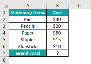
Enter the AutoSum function in cell B7. The below SUM formula appears automatically.
=SUM(B2:B6)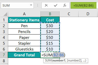
Press the Enter key. The function returns the result in cell B7 as $125, as shown below: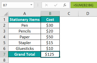
Thus, the AutoSum function adds all the numeric values in a given continuous range of cells.
Selecting the AutoSum function in Excel creates the SUM formula automatically to add the numeric values in a cell range.
It is a quicker way to use the AutoSum function. You need to hold the ALT key and click on the = key to enter the formula automatically.
Use this AutoSum In Excel Template to follow along with the examples in this article.
Download Excel TemplateRecommended Articles
Continue with these related resources when you want the next practical step in this topic.
- SUM Excel Function
- COUNT Excel Function
- COUNTA Excel Function
- COUNTBLANK In Excel
- SUBTOTAL Function In Excel
Explore the full Excel Counting and Summing Functions guide or browse Excel Resources.