RATE Function In Excel

What Is RATE Function In Excel?

The RATE Function in Excel calculates the rate of interest for paying the specified amount of a loan over a time period. The input provided to this formula is in integers, and the output is in percentages.

The RATE function is an inbuilt function in the Excel “Financial” category so that we can insert it from the “Functional Library” or directly enter it in the worksheet as a formula.

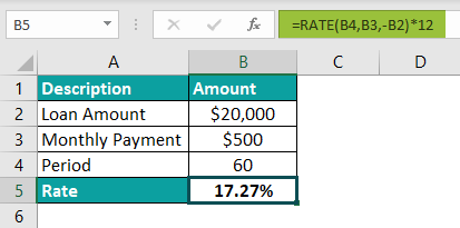
For example, we apply the RATE function to the present value of the loan amount ‘$20,000’, the monthly payment amount is ‘$500’, and the period is “5 years” to calculate the interest rate.

First, select cell B5, enter the formula =RATE(B4,B3,-B2)*12, and press the “Enter” key.

The output is ‘17.27%’, as shown above. We can see here that the input values are integers, and the formula returns a percentage output.

What Is RATE Function In Excel?

The RATE Function in Excel calculates the Interest rate, for a loan, over a time period.
Two factors commonly used by the finance industry are Cash outflow & Cash inflow. The Cash outflow is a negative number denoting the outgoing payments, and the Cash inflow is a positive number that denotes the incoming payments.
We can convert the number of periods to monthly or quarterly as per our requirement.
The function returns the output as 0. If there is no decimal value, we must format the cell value to the percentage format.

RATE() Excel Formula

The Syntax of the RATE Excel formula is,

The arguments of the RATE Excel formula are,

nper: It is a mandatory argument. It is the total number of periods over which the loan or investment is to be paid.
pmt: It is a mandatory argument. It is the payment for each period.
pv: It is a mandatory argument. It is the present value of all future payments.
fv: It is an optional argument. It is the future value that is the goal of the investment.
type: It is an optional argument. It is the formula that will consider the due dates for payments.
guess: It is an optional argument. It is the guess on the Interest Rate.

Excel VBA – All in One Courses Bundle (35+ Hours of Video Tutorials)

If you want to learn Excel and VBA professionally, then Excel VBA All in One Courses Bundle (35+ hours) is the perfect solution. Whether you’re a beginner or an experienced user, this bundle covers it all – from Basic Excel to Advanced Excel, Macros, Power Query, and VBA.

Start Learning Now

How To Use RATE Excel Function?

We can use the RATE Excel Function in 2methods, namely,

Access from the Excel ribbon.
Enter in the worksheet manually.

#Method 1 – Access from the Excel ribbon

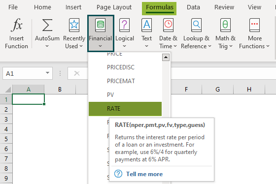
First, choose an empty cell > select the “Formulas” tab → go to the “Function Library” group → click the “Financial” option drop-down → select the “RATE” function, as shown below.

A “Function Arguments” window appears. Enter the value in the “nper,” “pmt,” “pv,” “fv,” “type,” and “guess” fields accordingly, and Press “OK”.

#Method 2 – Enter in the worksheet manually

Select an empty cell for the output.
Type =RATE( in the selected cell. [Alternatively, type “=R” and double-click the RATE function from the list of suggestions shown by Excel.
Enter the arguments as cell values or cell references.
Press the “Enter” key.

# Basic Example

Mr. Raj Mohan has taken a loan of $50,000 for five years. The installment amount of payment is $1,000. Let us calculate the Rate of interest using the RATE Excel Function.

In the table, the data is,

Column A contains a Description.
Column B contains Amount.

The steps to calculate the Interest Rate using RATE Function in Excel are as follows:

Select cell B8 and enter the formula =RATE(B4 i.e., the period, calculated as five years multiplied by 12, which gives 60.
Put a comma, and then select the cell that contains the installment amount, i.e., “B3”. Now, the formula will be =RATE(B4,B3
Put a comma, and then select the cell that contains the present value loan amount, i.e., B2. Now, the formula will be =RATE(B4,B3,-B2
Put a comma, and then select the cell that contains the future value, i.e., “B5”. Now, the formula will be =RATE(B4,B3,-B2,B5
Put a comma, and then select the value of the “type” argument as ‘1’. Now, the formula will be =RATE(B4,B3,-B2,B5,1
Put a comma, and then select the cell that contains the guess value, i.e., “B7”. Now, the formula will be =RATE(B4,B3,-B2,B5,1,B7
Finally, close the bracket and press the “Enter” key. The complete formula is: =RATE(B4,B3,-B2,B5,1,B7).

Mr. Raj Mohan’s interest rate is ‘2.21%’, as shown above.

Examples

We will understand some advanced scenarios using RATE Function in Excel.

#1 Example

Ms. Kathrine has taken a loan of $1,00,000 for five years. The future value of the amount is $2,00,000. Let us calculate the Rate of interest using the RATE in Excel.

In the table, the data is,

Column A contains a Description.
Column B contains Amount.

The procedure to calculate the Interest Rate using the RATE function in Excel is:

First, select cell B5, enter the formula =RATE(B4, ,-B2,B3), and press the “Enter” key.

[Cell B4 contains the period, the space for the installment argument is left blank, cell B2 contains the present value loan amount, and cell B3 contains the future value.]

The output is ‘14.87%’, as shown above.

#2 Example

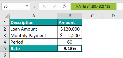
Mrs. Lorence has taken a loan of $1,20,000 for five years. The payment installment amount is $2,500. Let us calculate the Rate of interest using the RATE in Excel.

In the table, the data is,

Column A contains a Description.
Column B contains Amount.

The procedure to calculate the Interest Rate using the RATE function in Excel is:

First, select cell B5, enter the formula =RATE(B4,B3,-B2)*12, and press the “Enter” key.

[Cell B4 contains the period, cell B3 contains the installment amount, and cell B2 contains the present value loan amount.]

The output is 9.15%, as shown above.

#3 Example

XYZ company has borrowed $50,00,000 from the financial bank for ten years, and the payment installment amount is $5,000. Let us calculate the Rate of interest using the RATE function in Excel.

In the table, the data is,

Column A contains a Description.
Column B contains Amount.

The procedure to calculate the Interest Rate using the RATE formula in Excel is:

First, select cell B5, enter the formula =RATE(B4,B3,-B2)*12, and press the “Enter” key.

[Cell B4 contains the period calculated as ten years multiplied by 12, which gives 120, cell B3 contains the installment amount, and cell B2 contains the present value loan amount.]

The output is –33.05%, as shown below, i.e., the interest rate is calculated as negative.

Important Things to Note

The RATE function in Excel calculates using trial and error. After 20 iterations, an Error is returned.
To calculate the payment period’s interest rate, we can multiply by the number of months.
The positive numbers are used to represent cash inflows, and the negative numbers to represent cash outflows.
We can keep the “guess” argument as optional or ignore it, as it is just a starting value for an iterative procedure.

Frequently Asked Questions

What is the formula for the RATE function in Excel?

The RATE Function in Excel calculates the rate of interest for a specific period.

The formula for the RATE in Excel is as follows;

=RATE(nper,pmt,pv,[fv],[type],[guess])

In the following example, the formula is used to apply the RATE function to the present value of the loan amount ‘$1,00,000’, the monthly payment amount is ‘$1,000’, and the period is “10 years” to calculate the interest rate in cell B5. The formula is entered in cell B5. The complete formula is =RATE(B4,B3,-B2)*12, and the result is returned as ‘3.74%’, as shown below.

FAQ 1

Why is the RATE function Not Working?

The RATE Function in Excel is simple to use, but still, mistakes occur. The following are the errors that are the reasons for the function not working.

1. The “#NUM!” error occurs when the result or solution fails to execute.
2. The “#VALUE!” error occurs when some of the values in the arguments are not a number.

Where is the RATE function in Excel?

We can use the RATE Function in Excel as follows:

First, choose an empty cell → select the “Formulas” tab → go to the “Function Library” group → click the “Financial” option drop-down → select the “RATE” function, as shown below.

A “Function Arguments” window appears. Enter the value in the “nper,” “pmt,” “pv,” “fv,” “type,” and “guess” fields accordingly, and Press “OK”.

Download Template

This article must help understand the RATE Function in Excel formula and examples. You can download the template here to use it instantly.

RATE function in Excel Download

RATE Function In Excel