
What Is CAGR Formula In Excel?
CAGR, or Compound Annual Growth Rate, is an investment’s average yearly growth over a period of time that benefits those in finance and business. The CAGR Formula In Excel determines the rate of returns for an investment or asset over a time period, such as 3, 5, or 10 years. It uses the investment’s starting and ending balances as inputs, assuming that the profits get reinvested annually and the interest compounds annually.
Use this CAGR Formula In Excel Template to follow along with the examples in this article.
Download Excel TemplateKey Takeaways
- The CAGR function in Excel determines an investment’s average yearly growth rate, in other words, the rate of returns for an investment over a specific period.
- The CAGR formula in Excel takes the investment’s beginning and ending values to Calculate CAGR In Excel.
- We can also use the POWER(), RATE(), or IRR() functions to Calculate CAGR In Excel. However, when using the IRR(), all values except for the investment’s beginning and ending values should be 0.
- If we provide invalid arguments, the CAGR formula in Excel will return #VALUE! and #NUM! errors.
CAGR Formula In Excel
Excel does not have an inbuilt function to calculate CAGR. Hence, we will write a CAGR Formula In Excel or use functions such as POWER, RATE, and IRR.
The CAGR Formula In Excel is:
CAGR = (Ending Value / Beginning Value)(1/n) – 1
The arguments of the CAGR Formula In Excel are,
- Beginning Value – It is the first value in the investment.
- Ending Value – It is the last value in the investment.
- n – total number of periods. [Always remember that the years are not just calendar years but the completed years since we consider the year-end values].
For example, the below table shows the income details from 2010 to 2019. We will Calculate CAGR In Excel and display the output in cell B14.

Enter the formula =(B11/B2)^(1/9)-1 in cell B14.

The output is 4.99%, as shown above. The beginning value is 2000, the ending value is 3100, and the number of investing period is 9. Here, there are 10 years, but the time period is 9, i.e., 2010 to 2011, 2011 to 2012, 2012 to 2013, and so on.
[Note: The result will be in decimals. Since CAGR is a percentage-based value in the finance domain, we must change the cell format to Percentage, as depicted above].
How To Use CAGR Formula In Excel With Examples?
We can apply the CAGR formula in Excel using the following ways.
- Basic Method.
- Using the Power
- Using the RATE
- Using the IRR
#1 – Basic Method
We will Calculate CAGR In Excel using the Basic Method i.e., the CAGR formula in Excel.
In the below table, the data is,
- Column A contains Years.
- Column B contains Revenue for the years 2015 to 2021, respectively.

The steps to Calculate CAGR In Excel using the CAGR formula in Excel are:
Step 1: Enter the Beginning Value [cell B2], Ending Value [cell B8], and n in cells B11, B12, and B13, respectively.

Step 2: Enter the formula =(B12/B11)^(1/B13)-1 in cell B14.

The output is 12.25%, as shown above. The beginning value is 1000000, the ending value is 2000000, and the number of the investing period is 6.
#2 – Using the POWER Function
We will Calculate CAGR In Excel using the POWER function.
POWER() function – The function returns the value of a number when raised to a specific power.
The syntax of the POWER() function is:
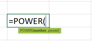
The arguments of the POWER() function are:
- number – It is the base value. It is a mandatory argument.
- power – The exponent. It is a mandatory argument.
In the below table, the data is,
- Column A contains Years.
- Column B contains Revenue for the years 2011 to 2021, respectively.

The steps to Calculate CAGR In Excel using the POWER function are:
Step 1: Enter the Beginning Value, Ending Value, and n, in cells E1, E2, and E3, respectively.

Step 2: Enter the formula =POWER(F2/F1,1/F3)-1 in cell F5.

The output is 3.24%, as shown above. The beginning value is 24000, the ending value is 33000, and the number of investing period is 10.
#3 – Using the RATE Function
We will Calculate CAGR In Excel using the RATE function.
RATE() function – The function determines the interest rate per annuity duration.
The syntax of the RATE() function is:

The arguments of the RATE() function are:
- nper – The total periods over which we need to pay an investment. It is a mandatory argument.
- pmt – The amount paid per period. It is a mandatory argument.
- pv – The current value of an investment. It is a mandatory argument.
- fv – The investment’s future value after NPER. It is an optional argument.
- type – It denotes when the installments are due. It is an optional argument.
- guess – It denotes our guess about the rate. It is an optional argument.
[Note: If we ignore the PMT value, we must provide the FV value. The argument type is 0 or 1, depending on the payments due at the end or start of the period. On the other hand, if we skip the argument guess, the formula will take a default value of 10%].
In the below table, the data is,
- Column A contains Years.
- Column B contains Revenue for the years 2008 to 2013, respectively.

The steps to Calculate CAGR In Excel using the RATE function are:
Step 1: Enter the nper, pv, and fv, in cells E1, E2, and E3, respectively. [We will ignore pmt and instead provide fv].

Step 2: Enter the formula =RATE(E1,,-E2,E3) in cell E6. [There is a blank in place of the 2nd argument as we have given values only for the 1st, 3rd, and 4th arguments].

The output is 6.59%, as shown above. The beginning value or PV is 2180, the ending value or FV is 3000, and the number of investing period or NPR is 5.
[Note: The argument PV is a negative number. Therefore, we must enter the function with the “-” sign, or else we will get #NUM! error].
#4 – Using the IRR Function
We will Calculate CAGR using the IRR excel function.
IRR() function – The function determines the internal rate of return for a cash flow sequence at uniform intervals.
The syntax of the IRR() function is:

The arguments of the IRR() function are:
- values – The data range that represents the cash flow series. It is a mandatory argument.
- guess – Our guess about the return rate. It is an optional value. [If we ignore it, the function takes the value as 10%].
In the below table, the data is,
- Column A contains Years.
- Column B contains Revenue for the years 2014 to 2020, respectively.

The steps to Calculate CAGR In Excel using the IRR function are:
Step 1: The starting value should be a negative figure, and all the entries between the investment’s beginning and ending values must be 0.

Step 2: Enter the formula =IRR(B2:B8) in cell B10.

The output is 2.90%, as shown above. The beginning value is -254500 (negative value), and the ending value is 302200].
CAGR Excel Errors
Few errors we get when applying the CAGR Function In Excel.
- #VALUE! – This Excel error occurs when we provide invalid arguments to the CAGR Function In Excel.
For instance, we will use the Basic Method to determine the CAGR in the below table.

The CAGR formula in Excel in cell B13 is =(B10/B9)^(1/B11)-1

However, we will get the error #VALUE! as shown below, as the ending value is a text instead of a numerical value.
- #NUM! – This error occurs when we do not provide the starting value argument as a negative value while using RATE() or IRR() to determine CAGR.
For instance, we will use the RATE() function to determine the CAGR in the below table.

First, we will enter the RATE() formula in cell B14 i.e., =RATE(B9,,B10,B11)

On the other hand, we will create an IRR function data of the table, which will be as shown below:
Then, we will enter the IRR() function in cell B11 i.e., =IRR(B2:B7)

Both the functions return the #NUM! error. However, once we provide the valid arguments, [ i.e., a negative beginning value], we will get the exact CAGR.
Important Things To Note
- The CAGR is a percentage value. So, when we apply the CAGR function in Excel, we must change the cell format, of the result cell, to Percentage.
- The arguments of the CAGR function in Excel should always be numerical values or cell references to numerical values but never a text value.
- When using the RATE() or IRR(), the beginning value must always be a negative number, or we will get #NUM! error.
Frequently Asked Questions (FAQs)
We can calculate CAGR in Excel using the below steps:
For example, the investment table to determine CAGR is shown below.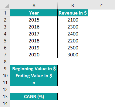
Step 1: Enter the Beginning Value, Ending Value, and Periods count in cells B9, B10, and B11, respectively.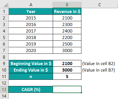
Step 2: Enter the formula =(B10/B9)^(1/B11)-1 in cell B13.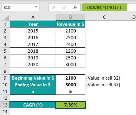
The output is 7.39%, as shown above. The beginning value is 2100, the ending value is 3000, and the number of investing period is 5.
We can calculate the future value or ending value from CAGR in Excel by:
1. Using the CAGR Basic Formula.
FV = PV * (CAGR + 1)n
Where,
FV – The future value or the investment’s ending value.
PV – The present value or the investment’s beginning value.
n – The number of periods.
2. Using Excel FV()
The syntax of the FV() function is: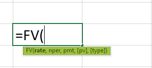
The arguments of the FV() function are:
rate – CAGR
nper – The total periods over which we need to pay an investment.
pmt – The amount paid per period.
pv – The current value of the investment
type – It denotes when the installments are due.
So, the FV() formula is =FV(rate, nper,,-pv,0) [The 3rd argument is blank, and the 4th argument is a negative number].
We use the CAGR function in Excel to determine various investments’ performances over time. The formula is helpful in finance and business domains.
Use this CAGR Formula In Excel Template to follow along with the examples in this article.
Download Excel TemplateRecommended Articles
Continue with these related resources when you want the next practical step in this topic.
Explore the full Excel Financial Functions guide or browse Excel Resources.