NOT Excel Function

What Is NOT Function In Excel?

The NOT Excel Function performs the set logical calculation first and then returns the reverse logical value of the result. If the calculation of the result is TRUE, we will get the output as FALSE, and vice versa.

The NOT Excel Function is an inbuilt Logical function, which means we can enter the formula directly in the worksheet or insert it from the “Function Library”.

For example, we will apply the NOT Function to calculate the logical value of the expression. Select cell A2, enter the formula =NOT(20>10), and press the “Enter” key.

The output is “FALSE”, as shown above.

[Output Observation: The result of the condition 20>10 is TRUE. Once the logical calculation is done, the TRUE reverses due to the NOT Excel Function and returns FALSE.]

What is NOT Function in Excel?

The NOT Excel Function checks the expression, evaluates the logical result as TRUE or FALSE, and then returns the reverse of the logical calculations result.
We get an Excel error if no argument values or cell reference is given.
The function argument uses cell references, numeric and text values, Boolean values, comparison operators, and other Excel functions. The argument evaluates the Boolean values of TRUE or FALSE or references or arrays containing logical values.
When the NOT function contains numeric value inputs, the zero evaluates to FALSE, and all other numbers, including negative numbers, evaluate to TRUE.

NOT() Excel Formula

The Syntax of the NOT Excel Formula is,

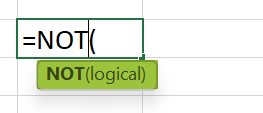
The argument of the NOT Excel Formula is,

logical: It is a mandatory argument. It is the value that evaluates TRUE or FALSE. If the expression is TRUE, the function returns FALSE, and if the expression is FALSE, the function returns TRUE.

Excel VBA – All in One Courses Bundle (35+ Hours of Video Tutorials)

If you want to learn Excel and VBA professionally, then Excel VBA All in One Courses Bundle (35+ hours) is the perfect solution. Whether you’re a beginner or an experienced user, this bundle covers it all – from Basic Excel to Advanced Excel, Macros, Power Query, and VBA.

Start Learning Now

How to Use NOT Excel Function?

We can use the NOT Excel Function in 2 methods, namely,

Access from the Excel ribbon.
Enter in the worksheet manually.

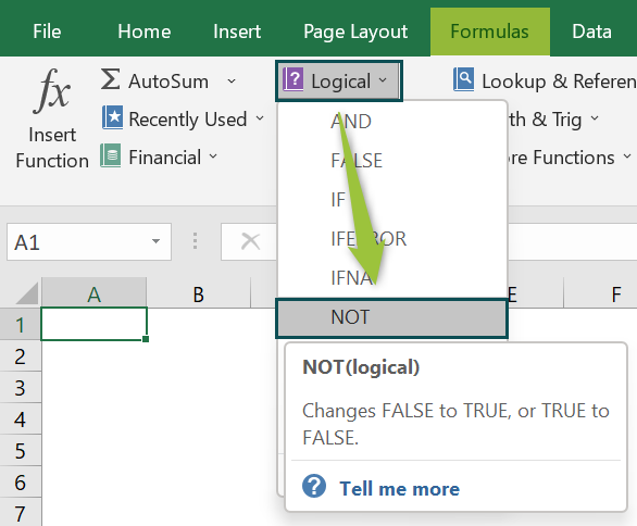
Method #1 – Access from the Excel ribbon

First, choose an empty cell → select the “Formulas” tab → go to the “Function Library” group → click the “Logical” option drop-down → select the “NOT” function, as shown below.

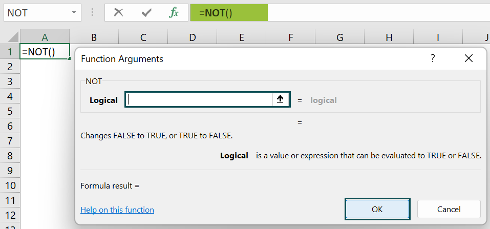
The “Function Arguments” window appears. Enter the argument in the “Logical” field → click “OK”, as shown below.

Method #2 – Enter in the worksheet manually

Select an empty cell for the output.
Type =NOT( in the selected cell. [Alternatively, type “=N” and double-click the NOT function from the list of suggestions shown by Excel.]
Enter the argument and close the brackets.
Press the “Enter” key.

Let us take an example to understand this function. We will calculate the logical values for the example of the student scores.

In the table, the data is,

Column A contains the Student Names.
Column B contains the Student Scores.
Column C displays the Output of the Logical Test.

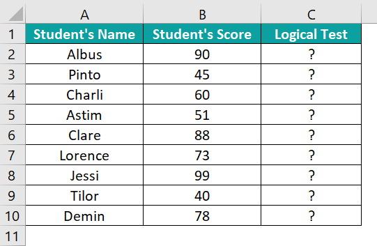
The steps to evaluate the values for the NOT Excel Function are as follows:

Select cell C2 and enter the formula =NOT(B2>60).
Press the “Enter” key. The result is “FALSE”, as shown below.

[Note: B2 cell’s value is 90, which is greater than 60. The logical result is “TRUE”, the formula reverses and returns “FALSE”.]
Drag the formula from cell C2 to C10 using the fill handle.

The output is shown above.

Examples

We will understand using NOT Function with some advanced scenarios.

Example #1

We will calculate the logical values using the NOT and the ISBLANK excel function.

In the table, the data is,

Column A contains the Value.
Column B displays the Output of the Logical Test.

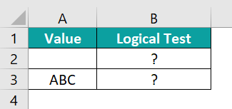
The steps to evaluate the values using NOT Function and ISBLANK() are as follows:

Step 1: Select cell B2 and enter the formula =NOT(ISBLANK(A2).

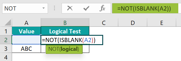
Step 2: Press the “Enter” key. The result is “FALSE” in the image below.

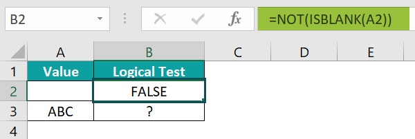
Step 3: Drag the formula from cell B2 to B3 using the fill handle. The output is shown below.

Example #2

We will calculate the logical value using the NOT Excel Function that returns an error as the output.

In the table, the data is,

Column A contains the Value1.
Column B contains the Value2.
Column C displays the Output of the Logical Test.

The steps to evaluate the values by the NOT Function are as follows:

Step 1: Select cell C2 and enter the formula =NOT(A2:B2).

Step 2: Press the “Enter” key. The result is a “#VALUE!” error, as shown below.

Example #3

We will calculate the logical values of an empty cell or ‘0’ value using the NOT Excel Function.

In the table, the data is,

Column A contains the Value.
Column B displays the Output of the Logical Test.

The steps to evaluate the values using the NOT Excel Function are as follows:

Step 1: Select cell B2 and enter the formula =NOT(A2).

Step 2: Press the “Enter” key. The result is “TRUE”, as shown below.

Step 3: Drag the formula from cell B2 to B3 using the fill handle. The output is shown below.

[Note: The empty/blank cell and 0 value display TRUE using the NOT Excel Function.]

Important Things to Note

The “#VALUE!” error occurs,
- When the given argument is neither a logical nor a numeric value.
- If none of the arguments evaluate logical values.
- If all of the values of the argument are empty cells.
The “#NAME?” error occurs if the function name is incorrectly typed.
If the NOT Excel function argument contains any empty cells, such values are ignored.

Frequently Asked Questions (FAQs)

1. What does the NOT function do in Excel?

The NOT Excel Function is an inbuilt function under the Logical Function of the Functional Library that operates under a logical test. The function is also called Boolean logic or function. The function is used as an individual function or part of the formula and other excel functions in a cell.

• If the value is TRUE, the NOT function returns FALSE.
• If the value is FALSE, the NOT function returns TRUE.

The syntax of the NOT function is =NOT(logical).

2. How to calculate the NOT Excel Function?

We can calculate the NOT Function as follows:

1.     Select an empty cell for the output.
2.     Type =NOT( in the selected cell. [Alternatively, type “=N” and double-click the NOT function from the list of suggestions shown by Excel.]
3.     Enter the argument and close the brackets.
4.     Press the “Enter” key.

For example, we will calculate the logical value using the NOT Excel Function.
The steps to evaluate the values by the NOT Function are as follows:

• Step 1: Select cell A2.

• Step 2: Next, enter the formula =NOT(A10=A1) and press the “Enter” key.

The result is “TRUE”, as shown above.

3. Where is the NOT Excel Function?

The NOT Excel Function is used as follows:

First, choose an empty cell → select the “Formulas” tab → go to the “Function Library” group → click the “Logical” option drop-down → select the “NOT” function, as shown below.

Download Template

This article must help understand the NOT Excel Function’s formula and examples. You can download the template here to use it instantly.

NOT Excel Function Download

NOT Excel Function