Excel Commands

What Are Excel Commands?

Excel commands enable one to perform mathematical calculations and statistical and logical operations in spreadsheets. And we can create an Excel command using inbuilt functions, which can vary from basic to advanced levels.

Users can use Excel commands to automate repetitive tasks and evaluations involving spreadsheet data, which always demand a result.

For example, the table below contains a list of students and their scores in Mathematics.

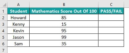
Suppose the requirement is to determine whether the students passed or failed in Mathematics, with 45 being the cut-off mark. Assume we must update the status in column C.

Then, we need to perform logical tests in column C. And the ideal way to do so is to use Basic Excel commands containing the IF() in the target cells, as depicted below.

In the above example, the IF() in each target cell checks if the Mathematics score in the corresponding column B cell equals or is more than 45. And if the condition holds in the target cell, the Excel command returns the TRUE value, PASS. Otherwise, the IF excel function output in the target cell will be FAIL.

Likewise, we can use other useful Excel commands to achieve the required outcomes per our requirements.

List Of Top 10 Excel Commands

Check out the following top ten Excel commands which can make our tasks involving spreadsheet data calculations and evaluations less tedious.

#1 – VLOOKUP Function To Fetch Data

Description

Suppose we need to find data in a table or a range by row. And the data to fetch could be in the same worksheet or different sheets. Then we can use Excel commands containing the VLOOKUP excel function to search and update the required data in the target cells.

The VLOOKUP() looks up a value in the leftmost column of the given table. And then, it returns the result in left-to-right order.

Example

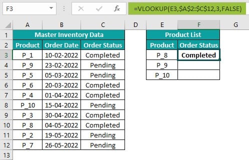
The table below shows two tables containing the master inventory data and a product list.

Suppose the requirement is to fetch the order status of products listed in the second table from the master inventory data table. Then, the common Excel commands used in such scenarios are those with the VLOOKUP().

Step 1: Select cell F3 and type the VLOOKUP() as shown below.

First, enter the equal to sign (‘=’), the function name, VLOOKUP, and an opening bracket.

We must enter the arguments mentioned in the VLOOKUP() syntax.

So, we enter the lookup_value, E3, the cell reference to the first product in the list.

Next, we enter a comma and the absolute reference to the source table range as table_array, $A$2:$C$12. And we do so as we require the formula with varying lookup values but the same source table data range.

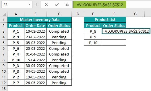
Then, we enter a comma and the Order Status column number in the source table as the col_index_num, 3.

And finally, we type a comma, after which Excel will show a drop-down list of options to set the range_lookup.

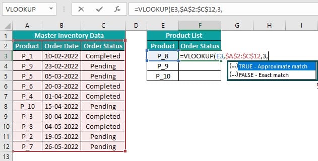
Let us set the match type as exact. So, double-click on FALSE to enter range_lookup. And enter the closing bracket to complete the command.

=VLOOKUP(E3,$A$2:$C$12,3,FALSE)

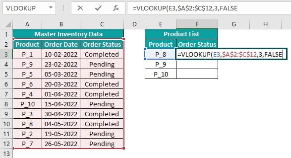
Step 2: Press Enter to view P_8’s order status in cell F3.

[Alternatively, the below command will also give the same result.

=VLOOKUP(E3,$A$2:$C$12,3,0)

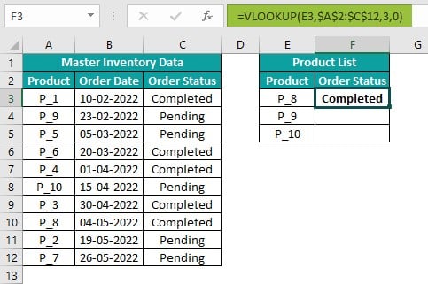
We can enter 0 as the last argument instead of entering FALSE or choosing FALSE from the drop-down list.]

Step 3: Using the excel fill handle, enter the command containing the VLOOKUP() in cell range F4:F5.

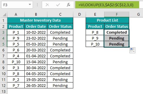
In the above example, each command looks for the exact match of each listed product’s (Column E) order status in the first table by the product name. And the function returns the required status based on the column C data.

Thus, we can use the VLOOKUP() as a standalone function to build basic Excel commands.

#2 – IF Condition To Do Logical Test

Description

The IF() makes the most common Excel commands that we can use to perform logical comparisons.

The function includes one or more test conditions. And if the specified conditions hold, the function returns the TRUE value. Otherwise, the IF() output in the target cell is the FALSE value.

Example

The table below shows items, their brands, and costs.

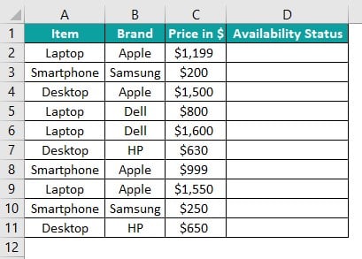
Suppose the requirement is to determine each product’s availability and display the status in column D. Assume the condition for an item’s availability is that its price should be equal to or below $1,000.

Then, in such cases, applying IF() in the target cells can fetch us the required information.

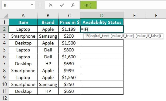
Step 1: Select cell D2 and enter the Excel command containing the IF() as shown below.

First, enter the equal to sign (‘=’), the function name, IF, and an opening bracket.

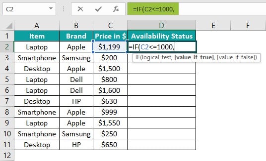
Next, enter the logical_test to check if the price in cell C2 is equal or is below $1,000, and then, enter a comma.

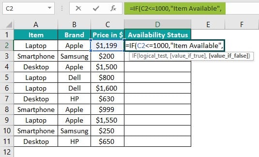
Next, enter the TRUE value to display when the condition holds, followed by a comma.

Finally, enter the FALSE value to display when the condition is false. And close the bracket to complete the command.

=IF(C2<=1000,”Item Available”,”Item Not Available”)

Step 2: Press Enter to view the availability status of the Apple laptop in cell D2.

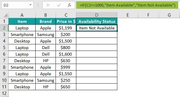
The IF() checks whether the Apple laptop price equals or is below $1,000. And as the condition is false, the function returns the FALSE value, Item Not Available.

Step 3: Using the fill handle, implement the IF() in the cell range D3:D11.

Likewise, we can create useful Excel commands using the IF() as a standalone function or with logical operators.

#3 – CONCATENATE Function To Combine Two Or More Values

Description

The CONCATENATE() based Excel commands join two or more text strings to form single strings.

The function can concatenate characters such as texts, numeric values, spaces, and special characters, with the output always being a text string.

Example

The table below shows a list of books and their authors.

Suppose the requirement is to display the book and author names in column C in the format shown in the column C heading. Then, the solution is to use CONCATENATE() based Excel commands.

Step 1: Select cell C2 and enter the CONCATENATE excel function as explained below.

First, enter the equal to sign (‘=’), the function name, CONCATENATE, and an opening bracket.

As per the function syntax, we must enter the texts to join, separated by commas.

So, enter the corresponding cell reference to the book name in row 2 as text1, followed by a comma.

Next, as per the format in cell C1, we must enter a space, a colon, and a space after the book name. So, provide the required text in double quotations as text2, followed by a comma.

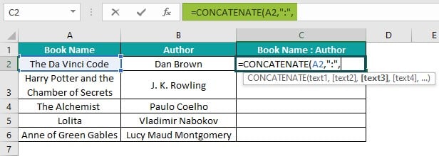
Finally, enter the corresponding excel cell reference to the author name in row 2 as text3 and a closing bracket to complete the command.

=CONCATENATE(A2,” : “,B2)

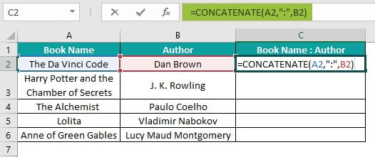
Step 2: Press Enter to view the CONCATENATE() output in cell C2.

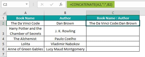
Step 3: Use the fill handle to update the CONCATENATE() in cell range C3:C6.

Thus, we achieve the data in the required format using the CONCATENATE().

Similarly, we can use the CONCATENATE function with other inbuilt functions to generate advanced Excel commands.

#4 – Count Only Numerical Values

Description

The Excel commands containing COUNT() can help when the requirement is to count only the number values in a data range.

The COUNT excel function counts cells containing numeric values, including date and time, provided the values have a valid numeric format. Otherwise, the function considers the values as texts and ignores them while counting numbers.

Example

The table below contains an employee’s details.

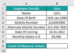
Suppose the requirement is to count cells containing only the numeric values in the employee details specified in the cell range B2:B7 and display the result in cell B9.

Then, applying the COUNT() based Excel command in cell B9 can help us obtain the required information.

Step 1: Select cell B9 and enter the COUNT() as explained below.

First, enter the equal to sign (‘=’), the function name, COUNT, and an opening bracket.

As per the function syntax, we must enter the values to check and count for cells containing numeric values.

So, we can enter the cell range B2:B7 as value1 or provide the cell reference to each cell in the cell range B2:B7, separated by commas as the function arguments. And enter a closing bracket to complete the command.

=COUNT(B2:B7)

Or

=COUNT(B2,B3,B4,B5,B6,B7)

Step 2: Press Enter to view the count of numeric values in the cell range B2:B7.

The function counts cell B4 and cells in the range, B6:B7 values as numbers. And thus, it returns 3 as the function output.

On the other hand, the COUNT() does not consider cells B3 and B5 data as numeric values, though they are a date and mobile number. The reason is that they should be in the proper formats for Excel to count them as numeric values. And the function considers them as texts.

#5 – Count All Values

Description

The Excel commands containing the COUNTA() can count non-empty cells in a given cell range.

The COUNTA excel function considers a cell as non-empty if it contains a text, numeric value, error value, empty string, or a formula returning the above-mentioned values.

Example

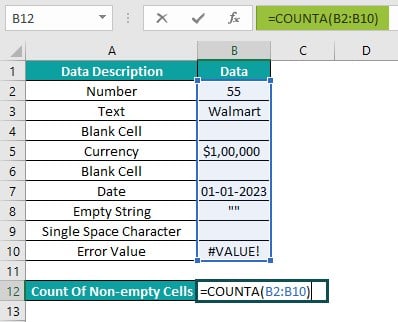
The table below contains a list of empty and non-empty cells in the cell range B2:B10, based on the data description in column A.

Suppose we need to count the non-empty cells in the cell range B2:B10 and display the result in cell B12. Then, applying an Excel command containing the COUNTA() in the target cell can generate the required result.

Step 1: Select the target cell B12 and enter the COUNTA() as explained below.

First, enter the equal to sign (‘=’), the function name, COUNTA, and an opening bracket.

As per the function syntax, we must enter the values to check and count for non-empty cells.

So, we can enter the cell range B2:B10 as value1 or provide the cell reference to each cell in the cell range B2:B10, separated by commas as the function arguments. And enter a closing bracket to complete the command.

=COUNTA(B2:B10)

Or

Step 2: Press Enter to view the count of non-empty cells in the cell range B2:B10.

The function counts all cells except B4 and B6. And thus, it returns 7 as the function output.

The reason is that cells B4 and B6 are blank. On the other hand, cell B9 appears to be empty. However, as mentioned in the description in the corresponding column A cell (cell A9), cell B9 contains a single space character. And thus, COUNTA() counts cell B9 as a non-empty cell.

#6 – Count Based On Condition

Description

Sometimes, we might have to count cells in a dataset based on a criterion. In such scenarios, we can use COUNTIF() based Excel commands.

The COUNTIF excel function counts the total number of cells meeting the specified condition.

Example

The table below contains a set of fruits and their quantities.

Suppose we must determine the count of fruits with 50 or more boxes and display the result in cell B9.

Then, an Excel command using the COUNTIF() in the target cell can get us the required data.

Step 1: Select the target cell B9 and enter the COUNTIF() as explained below.

First, enter the equal to sign (‘=’), the function name, COUNTIF, and an opening bracket.

As per the function syntax, we must enter the cell range and the criteria to check for cells where the specified criteria hold.

So, we can enter cell range B2:B7 as range, followed by a comma.

Next, we must enter the criterion as the criteria argument to check for cells in the range B2:B7, where the specified count of boxes equals or exceeds 50. We enter the criterion in double quotations as we must perform a logical test in excel. Otherwise, the criteria format will be different and depend on the conditions to check.

And then, enter a closing bracket to complete the command.

=COUNTIF(B2:B7,”>=50″)

Step 2: Press Enter to view the required cell count in cell B9.

The COUNTIF() checks for cells containing values that equal or exceed 50 in the cell range B2:B7. And as the given criterion holds in cells B2 and B5:B7, the function output is 4.

Furthermore, we can also use the COUNTIF() with wildcard characters (‘*’, ‘?’) in the criteria and complex criteria expressions to build advanced Excel formulas.

#7 – Count Number of Characters in The Cell

Description

Some tasks may require us to count the total characters in a cell. In such cases, we can use LEN() based Excel commands.

The LEN excel function accepts a text value in double-quotation or a cell reference to the text as input and returns the total number of characters in the specified string.

Also, the function counts the space characters, if present in the given text value.

Example

The table below shows a list of texts in column A.

Suppose we must count the number of characters in each cell in the range A2:A5 and display the result in the corresponding column B cells.

Then, applying the LEN() based Excel commands in cell range B2:B5 can fetch us the required data.

Step 1: Select the target cell B2 and enter the LEN() as explained below.

First, enter the equal to sign (‘=’), the function name, LEN, and an opening bracket.

According to the function syntax, we must enter the specified text in double quotations or a cell reference to the given text as input.

So, we will enter the reference to the corresponding column A cell A2 value, followed by a closing bracket to complete the command.

=LEN(A2)

Step 2: Press Enter to view the required character count in cell B2.

As the text “One” contains three characters, the LEN() output is 3.

Step 3: Use the fill handle to enter the LEN() in cell range B3:B5.

Thus, whether a character is a text, number, space character, or a special character, the LEN() counts it while determining the total number of characters in a cell.

#8 – Convert Negative Value to Positive Value

Description

Excel commands based on ABS() can be the apt solution for converting a negative value to a positive value.

The ABS excel function accepts a number or a cell reference to the number and returns its absolute value. In other words, it returns the number without its sign.

Example

The following table contains three negative values in column B.

Suppose we must convert them into positive values and display the output in column C. Then ABS() based Excel commands can fetch us the desired outcome.

Step 1: Select cell C2 and enter the ABS() as explained below.

First, enter the equal to sign (‘=’), the function name, ABS, and an opening bracket.

As per the function syntax, we must enter the given number or a cell reference to the given number as input.

So, we will enter the reference to the corresponding column B cell B2 value, followed by a closing bracket to complete the command.

=ABS(B2)

Step 2: Press Enter to view the required positive number in cell C2.

The ABS() accepts the value -50.25 as the input and returns the value 50.25 without the sign.

Step 3: Use the fill handle to enter the ABS() in cell range C3:C4.

Cell C4 output is a positive number but not a percentage as the input value.

But, we can select cell C4 and set the data format as Percentage in Home à Number Format to get the required percentage value.

Thus, the ABS() converts a negative number into a positive value, whether a percentage, currency, or in any valid number format.

#9 – Convert All Characters to UPPERCASE Values

Description

The Excel commands containing UPPER() are useful when converting the given texts to uppercase.

The UPPER excel function accepts a text or a cell reference to the text and returns the text in uppercase.

Example

The table below shows text values in column B.

Suppose the requirement is to change the given texts to uppercase and display the outcome in column C.

Then, the best solution is to use UPPER() based Excel commands in the target cells.

Step 1: Select cell C2 and enter the UPPER() as explained below.

First, enter the equal to sign (‘=’), the function name, UPPER, and an opening bracket.

As per the function syntax, we must enter the given text or cell reference to the given text as input.

So, we will enter the reference to the corresponding column B cell B2 value, followed by a closing bracket to complete the command.

=UPPER(B2)

Step 2: Press Enter to view the input text in uppercase in cell C2.

The UPPER() accepts the cell B2 text value, “uppercase text”, as the input and returns the text in uppercase, “UPPERCASE TEXT”.

Step 3: Use the fill handle to enter the Excel commands in cell range C3:C4.

Thus, irrespective of the case of the input text, the UPPER() returns the text in capital letters.

#10 – Find Maximum and Minimum Values

Description

While performing calculations in a worksheet, we may have to determine the maximum and minimum values in a given range. We can use MAX() and MIN() Excel commands in such scenarios.

The MAX and MIN functions accept a range of values or values separated by commas and return the largest and smallest number in the data range, respectively. The values can be named ranges, arrays, or cell references to numbers.

Further, the functions count logical values and numbers represented in the text when directly entered into the arguments list. On the other hand, they ignore blank cells, logical values, and texts in the given data range.

Example

The table below shows the Science test scores of ten students.

Suppose the requirement is to update the top and lowest scores in cell range C13:14 from the given list of scores.

Then, applying the MAX() and MIN() in cells C13 and C14 will fetch us the required data.

Step 1: Select cell C13 and enter the MAX excel function as explained below.

First, enter the equal to sign (‘=’), the function name, MAX, and an opening bracket.

As per the function syntax, we must enter the given cell range of values or values separated by commas as input.

So, we will enter the reference to the cell range containing the scores, C2:C11, followed by a closing bracket to complete the command.

=MAX(C2:C11)

Step 2: Press Enter to view the maximum score in cell C13.

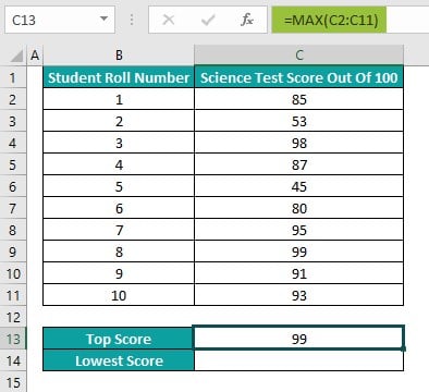
The MAX() accepts the cell range of Science test scores, C2:C11, and determines the highest score in the data range to return the output as 99.

Step 3: Select cell C14 and enter the MIN excel function as explained below.

First, enter the equal to sign (‘=’), the function name, MIN, and an opening bracket.

As per the function syntax, we must enter the given cell range of values or values separated by commas as input.

So, we will enter the reference to the cell range containing the scores, C2:C11, followed by a closing bracket to complete the command.

=MIN(C2:C11)

Step 4: Press Enter to view the least score in cell C14.

The MIN() accepts the cell range of Science test scores, C2:C11, and determines the lowest score in the data range to return the output as 45.

Download Template

This article must be helpful to understand the Excel Commands, with its formula and examples. You can download the template here to use it instantly.

Recommended Articles

This has been a guide to Excel Commands. Here we explain the top ten excel commands with examples and downloadable excel template. You may learn more from the following articles –

• Divide In Excel
• Excel Subtraction Formula
• Status Bar In Excel