Excel Subtraction Formula

What Is Subtraction Formula In Excel?

The Subtraction formula in Excel performs the subtraction arithmetic operation. It finds the difference between the specified values. The simple Excel Subtraction formula uses the minus sign (‘–‘) to subtract one number from another. However, users can use the formula to subtract values such as percentages, dates, times, matrices, texts, and lists.

For example, the following table contains two values’ sets and the commands to execute using the values specified in corresponding rows.

Assume we need to apply the required formulas in column D. Then, considering the Excel Subtraction formula meaning explained above, we can apply the Subtraction formula in the target cells as depicted below.

In the above Excel Subtraction formula example, each expression in every target cell uses the minus sign to execute the required subtraction operation.

Thus, we can use the Excel Subtraction formula for multiple cells with different requirements, as shown in the above example.

How To Use Subtraction Formula In Excel?

The steps to use the Excel Subtraction formula in Excel are as follows:

1. First, check if the values we need to subtract are valid and correct.
2. Next, choose the target cell and enter the required Excel Subtraction formula.
3. Finally, press Enter to view the difference value.

The below example explains the Excel Subtraction formula meaning and the abovementioned steps in detail.

The following table contains six-month monthly income and expense data.

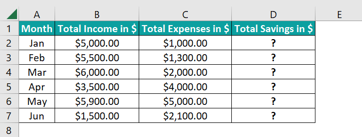
Suppose the requirement is to determine the monthly savings based on the given income-expense data and display the result in column D.

Then, it is an example of the Excel Subtraction formula whole column, and applying the Subtraction formula in the target cells will fetch us the required savings data.

Examples

Check out the below Excel Subtraction formula examples to use the formula effectively.

#1 – Subtract Cells In Excel

The following Excel Subtraction formula example shows the different ways of subtracting Excel cells.

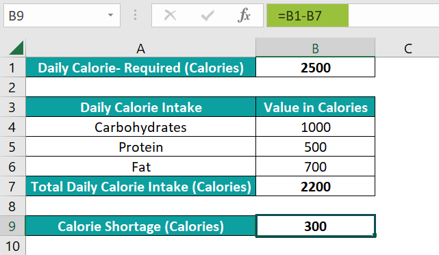
The below image shows the calorie data of a person.

Cell B contains the required daily calories, 2500. The cell range A3:B7 shows the daily calorie intake breakdown, and cell B7 shows the total daily calorie intake as the sum of the calories contributed by the three nutrients, 2200.

Suppose the requirement is to determine the calorie shortage as the difference between the daily calorie required and total intake and display the output in cell B9. Then, here is how you can apply the Subtraction formula in the target cell and get the required data.

• Step 1: Select the target cell B9, enter the below formula, and press Enter.

=B1-B7

Alternatively, the below formulas will get you the same results.

=B1-B4-B5-B6

Or

=B1-SUM(B4:B6)

In all the above formulas, the minus sign precedes the values we aim to subtract from the required daily calorie value of $2,500. And the above three formulas show the different ways to represent the subtrahend or the total daily calorie intake value in the formulas.

#2 – Subtract Columns

Let us see how to use the Excel Subtraction formula to subtract columns.

The first table contains the marked and selling price details for five items.

And the second table shows the reduction factor of $100 for the marked prices specified in the first table as a holiday offer.

Suppose we must determine the discount amounts for the items in the first table as the difference between the respective marked and selling prices. And then, determine the revised marked price for each item in the second table based on the specified reduction factor. Assume the target cells are D2:D6 and G4:G8 for the first and second requirements, respectively.

Then, here are the steps to achieve the required outcome using the Subtraction formula in the target cells.

• Step 1: Select the target cell D2, enter the below formula, and press Enter.

=B2-C2

• Step 2: It is a scenario of the Excel Subtraction formula whole column. Thus, using the fill handle, update the formula in cell range D3:D6.

Thus, the Subtraction formula in the target cells returns the discount amount on each item based on the respective marked and selling prices.

• Step 3: Select the target cell G4, enter the below formula, and press Enter.

=B2-$F$2

• Step 4: We can use the above Excel Subtraction formula for multiple cells, G5:G8, by dragging the Excel fill handle downwards.

The above Subtraction formula deducts cell F2 value, $100, from the marked prices provided in column B to get the revised marked prices in cell range G4:G8.

Thus, the above example shows how to subtract columns and deduct one constant value from the chosen cells in a column.

#3 – Subtract Percentage

The below illustration shows how to apply the Excel Subtraction formula to subtract percentages.

The first table contains two percentages, and the requirement is to determine and display the difference between them in cell C2.

On the other hand, the second table contains the grocery purchase amount and the discount % on it. And the requirement is to determine and show the final billing amount after the discount deduction from the purchase amount in cell C5.

Then, here are the steps to apply the Subtraction formulas in the target cells and achieve the required output.

• Step 1: Select the target cell C2, enter one of the below Subtraction formulas, and press Enter.

=A2-B2

Or

=50%-10%

• Step 2: Select the target cell C5, enter one of the below Subtraction formulas, and press Enter.

=A5*(1-B5)

Or

=500*(1-15%)

The cell C2 Subtraction formula finds the difference between the two specified percentages to return the difference as a percentage, 40%.

On the other hand, the cell C5 Subtraction formula calculates 15% of the purchase amount, $500. And then, it deducts the result from the purchase amount to return the final billing amount as $425.

#4 – Subtracting Dates

The following Excel Subtraction formula example explains how the formula helps subtract date values.

The two tables below show an order’s dispatch and receive date data.

However, the second table includes the informed revised dispatch date details.

Suppose the requirement is to determine the order delivery duration in cell D2 based on the data specified in the first table. And then, calculate the actual order receive date, based on the data provided in the second table, in cell E6, which has the data format set as Date in Home → Number Format.

Then, the steps to apply the Subtraction formulas in the two target cells and obtain the required data are as follows:

• Step 1: Select the target cell D2, enter the below formula, and press Enter.

=C2-B2

Alternatively, we can enter the dates using the DATE Excel function in the Subtraction formula and get the above result.

=DATE(2022,3,21)-DATE(2022,3,11)

The above formulas subtract the smaller date (3/11/2022) from, the bigger date (3/21/2022) to return the number of days between them, 10.

• Step 2: Select the target cell E6, enter the below formula, and press Enter.

=C6-B6+D6

We can also use the DATE() as explained in the previous step or apply the DATEVALUE Excel function instead of supplying the Excel cell references to the dates in the cell E6 Subtraction formula.

=DATEVALUE(“3/21/2022”)-DATEVALUE(“3/11/2022”)+DATEVALUE(“3/15/2022”)

The above formulas first compute the delivery duration for the given date values in cell range B6:C6, 10. But as the dispatch date got revised, adding the revised date to the calculated duration returns the new or actual order receive date, 3/25/2022.

#5 – Subtracting Times

Let us see how to use the Excel Subtraction Formula to subtract time values.

The below table contains the entry and exit times of a worker in a firm.

Suppose we must determine the working time the worker clocked each day based on the given timesheet data and display the results in column D.

Then, applying the Subtraction formula as explained below will get us the required timesheet data.

• Step 1: Select the target cell D2, enter the below formula, and press Enter.

=C2-B2

Using the TIMEVALUE Excel function instead of the cell references to the time values in the Subtraction formula will also give the same result.

=TIMEVALUE(“18:30”)-TIMEVALUE(“9:30”)

• Step 2: Using the fill handle, implement the formula in cell range D3:D6.

The Subtraction formula in each target cell subtracts the entry time from the exit time to return the working duration the worker clocked each day.

For example, the cell D6 formula finds the duration between 22:00 (10 pm) and 16:05:00 (4:05 pm), which is 5:55 (5 hours and 55 minutes). Thus, the worker clocked 5 hours and 55 minutes on 12/2/2022.

#6 – Matrix Subtraction

Here is an illustration to show how the Excel Subtraction formula helps perform matrix subtraction.

The below image shows two matrices, Matrix 1 and Matrix 2.

Suppose the requirement is to determine the difference between the two matrices and display the results in the third matrix. Then applying the Subtraction formula in each cell in the third matrix cell range will fetch us the required data.

• Step 1: Select the target cell F4, enter the below formula, and press Enter.

=B2-B7

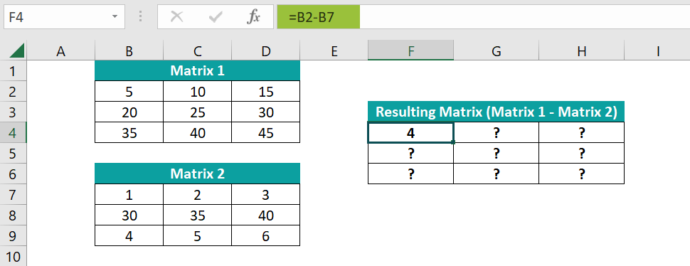
• Step 2: Drag the fill handle downwards till cell F6 and then to the right till cell H6 to apply the formula in the remaining cells of the third matrix.

Let us see the cell H6 expression to check how the formula works. The formula subtracts the cell D9 value, 6, from the cell D4 value, 45, to return the difference as 39.

Alternatively, we can select the cell range F4:H6 and enter the Subtraction formula as an array formula.

• Step 1: Select the cell range F4:H6 and enter the below formula.

=B2:D4-B7:D9

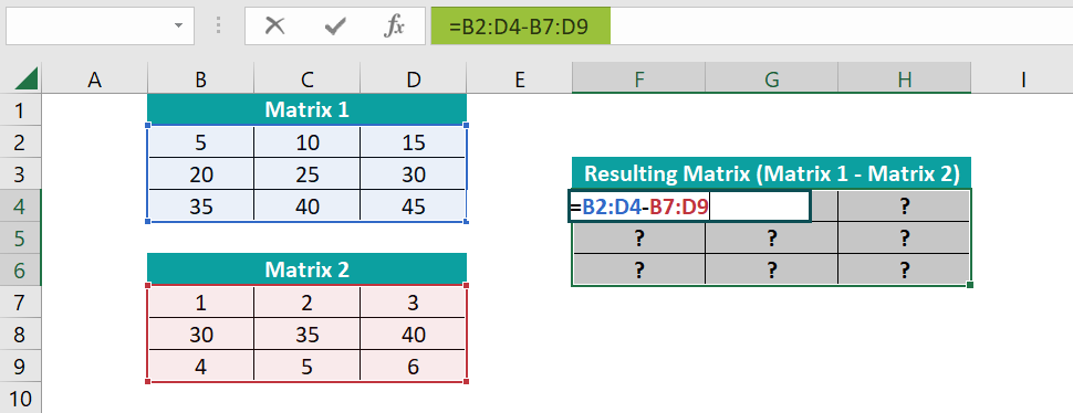
• Step 2: Press the keys Ctrl + Shift + Enter to apply the above expression as an array formula in Excel.

{=B2:D4-B7:D9}

#7 – Subtract Text Of One Cell From Another Cell

All the previous Excel Subtraction formula examples dealt with subtracting numeric values.

We shall now see how to apply the Subtraction formula to subtract a text value of one cell from another cell.

The below table contains a list of employee names.

Suppose the table contains the text to subtract from the corresponding employee name in each row and display the resulting text in column D.

Then, as this is a scenario of case-sensitive subtraction, applying the following Excel Subtraction formula in the target cells will help us obtain the required texts.

• Step 1: Select the target cell D2, enter the below formula, and press Enter.

=TRIM(SUBSTITUTE(B2,C2,””))

• Step 2: Using the fill handle, implement the above expression in cell range D3:D5.

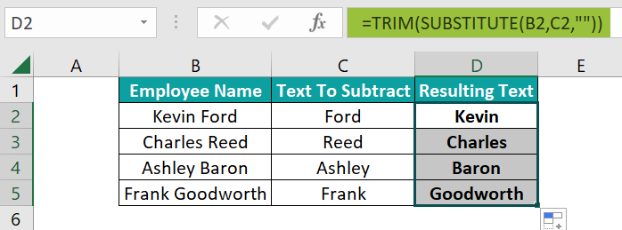
Let us see the cell D5 expression to check how the formula executes. First, the SUBSTITUTE Excel function replaces the text specified in cell C5, Frank, with a space in the cell B5 text, Frank Goodworth. And then, the TRIM in Excel removes the spaces in the resulting text, thus returning the required text as Goodworth.

But, assume column C contains the below texts to subtract from the respective employee names.

It is a scenario of case-insensitive subtraction. Hence applying the below Subtraction formula will get us the required outcome.

• Step 1: Select the target cell D2, enter the below formula, and press Enter.

=TRIM(REPLACE(B2,SEARCH(C2,B2),LEN(C2),””))

• Step 2: Next, enter the above formula in cell range D3:D5 using the fill handle.

In the above cell D5 formula, the LEN Excel function returns the cell C5 text string length, 5. Next, the SEARCH() searches the cell C5 text, frank, in cell B5 to return the text position in the cell B5 text as 1. Then, the REPLACE Excel function replaces five characters in the cell B5 text, starting from the first character with “”. And finally, the TRIM() removes blank space before the resulting text to return the remaining text, Goodworth.

#8 – Subtract One List From Another

The below example shows how the Excel Subtraction formula helps subtract a given list from another.

The table below contains the richest US states and states with the highest cost of living lists.

Suppose we must determine the richest states, not with the highest cost of living, and display the results in column D. Then, we can use the following Subtraction formula in the target cells to achieve the required data.

• Step 1: Select the target cell D2, enter the below formula, and press Enter.

=IF(COUNTIF($C:$C,$B2)=0,”Yes”,”No”)

• Step 2: Drag the fill handle downwards to enter the formula in cell range D3:D8.

Consider the cell D8 expression to understand how the formula executes. First, the COUNTIF Excel function checks the cell B8 value, Washington, in column C. As it occurs in column C, once, in cell C4, the COUNTIF() returns 1.

So, the IF condition does not hold in cell D8, as the COUNTIF() return value of 1 is not equal to 0. And thus, the IF() returns the FALSE value, No.

On the other hand, B3:B5, the cell range’s values do not appear in column C. Hence, the IF conditions in their corresponding target cells hold. And thus, the IF functions in these three rows (cell range D3:D5) return the TRUE value, Yes, as the output.

Important Things To Note

• Excel does not provide an inbuilt function to perform subtraction in Excel. But we can create an Excel Subtraction formula using the minus sign, ‘–‘.
• Ensure the values we subtract are of the same data type to avoid potential errors. For example, when subtracting numeric data, if one value is text, it can result in an error value.
• Be careful while using the minus sign with other arithmetic operators. Excel will execute them in a particular order, starting from brackets, division, multiplication, addition, and subtraction.

Frequently Asked Questions (FAQs)

Download Template

This article must be helpful to understand the Excel Subtraction Formula, with its formula and examples. You can download the template here to use it instantly.

Recommended Articles

A guide to Excel Subtraction Formula. Here we learn to use the subtraction formula with step-by-step examples & downloadable excel template. You can learn more from the following articles –

• Excel Minus Formula
• Percentage Change Formula In Excel
• ABS Excel Function