What Is Minus Formula In Excel?
The Excel Minus Formula subtracts numbers with the supplied value. It is built with the Minus “-” Operator. It is not an inbuilt formula and for the completion of the formula, the Equal to sign is also included. The Minus Formula in Excel is written as “=Value 1 – Value 2.” This means that value 2 is subtracted by value 1.
For example, consider the below table with two values in column A. We need to use the below steps to obtain the result with Minus Formula. The steps used to find the subtracted value in Excel are as follows:
📥Download the ready-to-use Excel template to practice this tutorial yourself.
Excel Minus Formula
- To begin with, select the cell to display the result. In this example, we have selected cell A3.
- Next, enter the formula in cell A3.
- The complete formula is =A1-A2.
- Then, press Enter key. The output is returned as 10 in cell A3

Likewise, we can obtain the subtracted value using Excel Minus Formula.
Table of contents
Key Takeaways
- The numbers or cell references can be entered directly when using the Excel Minus formula.
- The Excel Minus Formula is applied on percentage formatting in case of decimal results.
- The basic rules of Mathematics such as the BODMAS rule is followed in this formula.
- It is the easiest method to subtract time and get its differences.
- The Minus Formula method we have covered will work with all the versions of Excel.
How To Use Minus Formula In Excel? (With Steps)
We can enter the function in the worksheet directly with the below steps;
- Type = for entering the Minus Formula in Excel.
- Select Value 1.
- Enter the ‘-’ Operator.
- Select Value 2.
- Press Enter key to obtain the result.
Basic Example
The below table shows two values, one in cell A2 and the other in cell B2. We need to use the following steps to find the subtracted value by inserting Minus Formula.
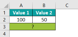
The steps to obtain the result with Minus Formula in Excel are as follows:
Step 1: Select an empty cell to display the output. We have selected merged cells A3 and A4 in this case.
Step 2: Enter the Minus Formula in Excel.
The complete formula is =A2-B2
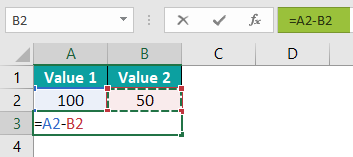
Step 3: Press Enter key.
We can see that the function has returned the value of 50.
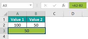
Likewise, we can find the subtracted value using minus formula.
Excel Minus Formula Examples
Let us look at the following examples to understand the formula.
Example – #1
The below table shows the selling price and cost price of fruits. First, we need to calculate profit from the values with Minus Formula in Excel.
In the table,
- Column A lists the Fruits
- Column B contains the Cost Price
- Column C shows the Selling Price
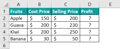
The steps used to find the subtracted values using Minus Formula in Excel are as follows:
Step 1: Select an empty column to display the output. We have selected column D in this case.
Step 2: Enter the Minus Formula.
The complete formula is =C2-B2.
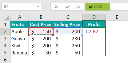
Step 3: Press Enter key.
The image below shows the results in cell D2, as the minus of the numbers is $50.
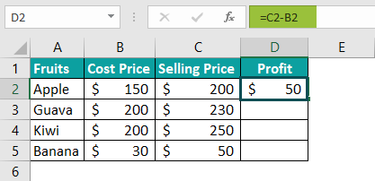
Step 4: Drag the AutoFill arrow to D5 to obtain subtracted values in other cells.

Similarly, we can use Excel minus formula to obtain results.
Example – #2
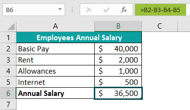
The below table shows the employee’s annual salary. We need to calculate the total annual salary from the values using Minus Formula in Excel.
In the table, the data is reflected as below:
- Column A contains the Detail of the Salary of Employees
- Column B contains the Amount
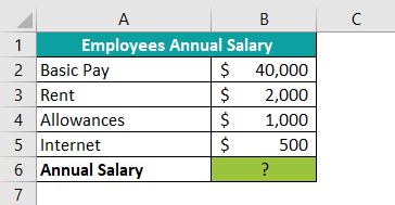
The steps used to obtain results by inserting minus formula are as follows:
Step 1: Select an empty cell to display the output. We have selected cell B6 in this case.
Step 2: Enter the complete formula, =B2-B3-B4-B5
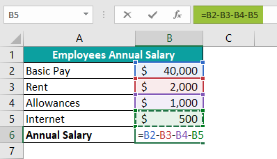
Step 3: Press Enter key.
The function has returned the result as $36,500 in cell B6 by subtracting all values from Basic Pay.
Likewise, we can obtain values with Minus formula.
Example – #3
The table shows a few companies’ sales and purchases data in columns A, B and C respectively. We need to calculate turn over profit from the values with Minus Formula in Excel.

The steps used to find values with Excel Minus formula are as follows:
Step 1: Select an empty column to display the output. We have selected column D in this case.
Step 2: Enter the Minus Formula in Excel.
The complete formula is =C2-B2
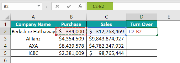
Step 3: Press Enter key. We can see that the function has returned the result as $312,434,469 in cell D2.

Step 4: We can manually enter the formula in all the cells or use the AutoFill option. Let us use the AutoFill option. Drag the cursor to cell D2. We can see the results instantly.

Similarly, we can use the function to subtract values in excel.
Important Things To Note
- The Excel Minus Formula is one of the four basic arithmetic operations.
- Unlike the SUM Excel function, there is no inbuilt function of the Minus formula in excel.
- We can subtract any value, like; numbers, percentages, days, months, hours, minutes, and seconds. We can also subtract matrices, text strings, and lists.
- The data format used for subtracting the time should be in TIME format, i.e., HH: MM format or MM: SS format, depending on the requirements.
- It is used for calculating or subtracting the difference in any number type.
- The formula doesn’t give the actual time difference by subtracting; instead, converting it to another format is required.

Frequently Asked Questions (FAQs)
The below table shows the values in percentage. We will calculate the output in percentage from the values using Minus Formula in Excel.
The steps used to find values with excel minus formula are as follows:
Step 1: Select an empty cell to display the output. We have selected cell C2 in this case.
Step 2: Enter the Minus Formula
The complete formula is =A2-B2
Step 3: Press Enter key. The function has returned the result as 60% in cell C2 by subtracting numbers in percentage.
We can calculate the output in percentage in excel minus function.
For example, the below image shows the dates. We will calculate the output from the dates using Minus Formula in Excel.
In the table, the data is reflected as below:
a. Column A contains the Start Date
b. Column B contains the End Date
The steps to demonstrate the Minus Formula are as follows:
1. Select an empty cell for the output. We have selected cell C2 in this case.
2. Enter the Minus Formula in Excel. The complete formula begins with the “=” sign. Then, select End date as “B2”, enter the “-” sign, and then select Start date as “A2”.
3. The image below shows the results in cell C2; by subtracting dates, the result is obtained as ‘27 days.’
For example, the below image shows the time in hours, minutes, and seconds. We will calculate the output from the time using Minus Formula in Excel.
In the table, the data is reflected as below:
a. Columns A, B, & C contains Time 1 in Hours, Minutes, & Seconds.
b. Columns E, F, & G contains Time 2 in Hours, Minutes, & Seconds.
c. Columns in C, D, & E in Row 4, contain the output, i.e., Minus of two Times, Time 1 And Time 2 in Hours, Minutes, & Seconds.
The steps to demonstrate the Minus Formula are as follows:
1. Select empty cells for the output. We have selected cells C4, D4, and E4 in this case.
2. Enter the Minus Formula in Excel. The complete formula is is {=(A2:C2)-(E2:G2)}.
3. Select cells C4, D4, and E4, and press CTRL + SHIFT + ENTER.
4. The image below shows the results in cells C4, D4, and E4; by subtracting times, the result is ‘90 180 270.’
Download Template
📥Download the ready-to-use Excel template to practice this tutorial yourself.
Excel Minus FormulaRecommended Articles
This has been a guide to Excel Minus Formula. Here we discuss how to use minus formula with examples and downloadable excel template. You can learn more from the following articles –

Leave a Reply