
What Is RIGHT Function In Excel?
The RIGHT function in Excel is an inbuilt TEXT function that returns the characters from the right end of a text string based on the specified number of characters. Users can use the RIGHT() to get the required characters from the given text string while performing financial analysis. Also, the function shows impressive results when used with Excel functions, such as SUM, SEARCH, and LEN.
For example, the below table shows five sample texts.
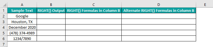
We can use the RIGHT() in all the cells in column B to display only the required characters from the right side of the specific text string, as depicted in the below image.
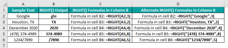
In the above RIGHT function in Excel example, column B shows the number of characters specified in the RIGHT() function to display as the output in each cell. And columns C and D show the two ways we can provide the arguments to the RIGHT function in Excel to achieve the same results.
📥Download the ready-to-use Excel template to practice this tutorial yourself.
RIGHT Function In ExcelTable of contents
Key Takeaways
- The RIGHT function in Excel extracts a specified number of characters from the end of a given text string. We can achieve excellent results using the RIGHT() with Excel functions such as SEARCH and LEN.
- The RIGHT function in Excel syntax is =RIGHT(text,[num_chars]), where text is the mandatory argument and num_chars is an optional argument.
- When we do not specify the num_chars argument in the RIGHT(), it takes the default value of 1.
- If we want to show a date value as a text, ensure the source text string has the Number Format as Text. Otherwise, the RIGHT() will return a number equivalent to the specific date.
RIGHT() Excel Formula
The RIGHT function in Excel syntax is:
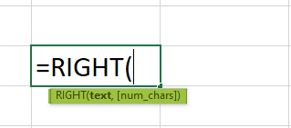
where,
- text: It is the mandatory argument and denotes the text string provided as the source data.
- num_chars: It is an optional argument, indicating the number of characters to extract from the right end of the provided text string.
When we do not specify the num_chars argument in the RIGHT(), it takes the default value of 1.
On the other hand, if the argument num_chars is a value more than the given text string length, the RIGHT() will return the entire text as the output. And if the argument num_chars is a value below zero, the RIGHT() will return the #VALUE! error.
Please Note: The RIGHT function in Excel counts a character as 1, irrespective of the default language setting and whether the character is single- or double-byte.
How To Use RIGHT Excel Function?
The steps to use the RIGHT function in Excel are:
- First, ensure the text strings in the source data are accurate and complete.
- Then, select the target cell and enter the RIGHT().
- Press Enter key and copy the formula into cells where we have to display the specified set of characters from the right side of other text strings in the source data.
The following example will help us understand the RIGHT function in Excel definition and the above steps.
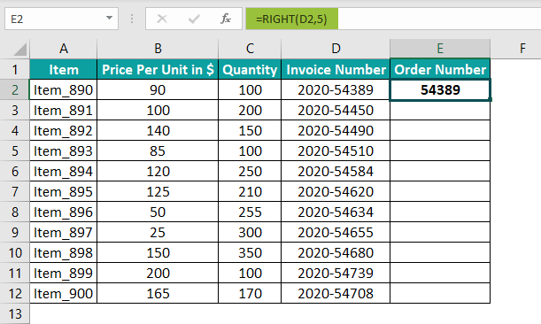
Assume we have a table containing eleven items’ order and invoice details.
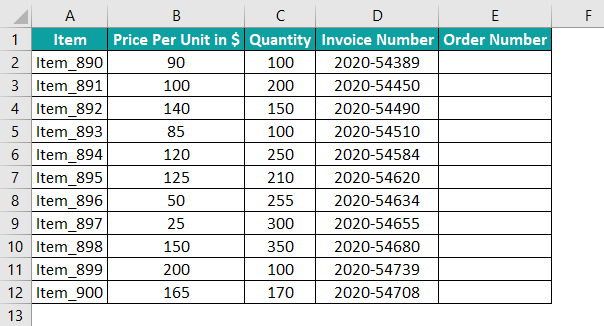
And we require to extract the order numbers from the invoice numbers and populate column E. Then, we can use the RIGHT() to display the required characters from the right end of each invoice value.
Step 1: Select cell E2, enter the following RIGHT(), and press Enter.
=RIGHT(D2,5)
Alternatively, we can select cell E2 and choose Formulas > Text > RIGHT to open the Function Arguments window.
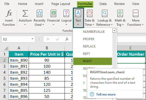

We can now enter the arguments’ values in the Function Arguments window and click OK to get the RIGHT() output in cell E2.
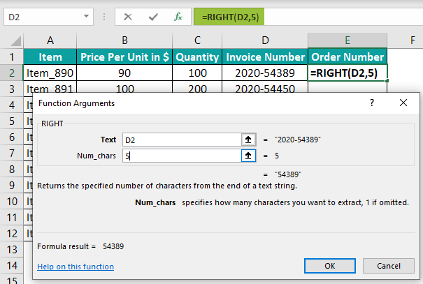
The Function Arguments window shows the RIGHT function in Excel definition, each argument value, and the result that will display in the target cell.
Step 2: Drag the fill handle downwards to copy the formula in the cell range E3:E12.

Please Note: Since the order number in each invoice value is of the same length, 5, the second argument remains the same in all the cells containing the RIGHT(), E2:E12. Otherwise, the RIGHT() formula would differ for each cell based on the two specified arguments.
Examples
Here are a few examples to effectively understand the RIGHT function in Excel.
Example #1
Consider the below table containing text strings.
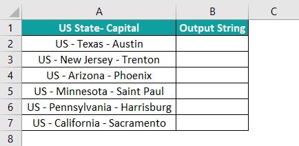
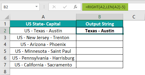
Suppose we want to display only the state-capital data in each cell from B2:B7. Therefore, we need to remove the term ‘US – ‘ from each text string.
Typically, we would enter the RIGHT() with different arguments’ values in each cell. Instead, we can use the RIGHT() with the LEN() Excel function.
The formula will remove a specific fixed number of starting characters from the text strings and display the required characters from their right end.
The steps used to display specific data from the table are:
Step 1: Select cell B2, enter the below formula containing the RIGHT() and LEN(), and press Enter.
=RIGHT(A2,LEN(A2)-5)
Step 2: Drag the fill handle downwards to copy the formula in cell range B3:B7.
In the above RIGHT function in Excel example, the cell reference to the specific text string is the first argument value in the RIGHT() in each cell. And the LEN() defines the second argument, num_chars, as the total length of the specific text string without the first five characters (U, S, ” “, “–“, ” “).
Thus, our formula remains the same in cells B2:B7, with only reference to the specific text string change in each cell.
Example #2
Consider the below table. It shows a list of dates with their Number Format as Text. Suppose we need to extract the year from each text string and display the output in column B.
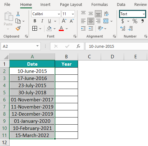
Please Note: If the dates have the Number Format as General or Date, the RIGHT function in excel for dates will return a number equivalent to each year.
But since, in the above example, the dates are text values, we can apply the RIGHT function in Excel and achieve the results.
Step 1: Select cell B2, enter the RIGHT() mentioned in the Formula Bar in the below image, and press Enter.
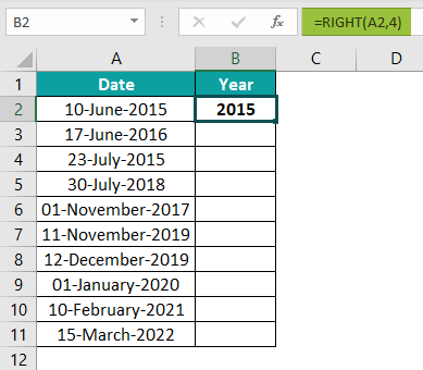
Step 2: Drag the fill handle downwards to copy the formula in cell range B3:B11.
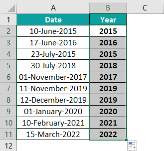
Here, the number of characters we need to display in column B from the right side of each text string is 4.
So, the second argument in the formulas used through the range B2:B11 for the RIGHT function in Excel for dates remains the same.
Example #3
Typically, the RIGHT function in Excel returns a number extracted from a text string as a text. Here is an example of how we can use the RIGHT() with the VALUE() to get the numeric data in the correct format.
Suppose we need to extract the ZIP Code from the text strings in column A in the below table as numbers.

Then, the steps are:
Step 1: Select cell B2, enter the below formula containing the RIGHT() and VALUE(), and press Enter.
=VALUE(RIGHT(A2,5))
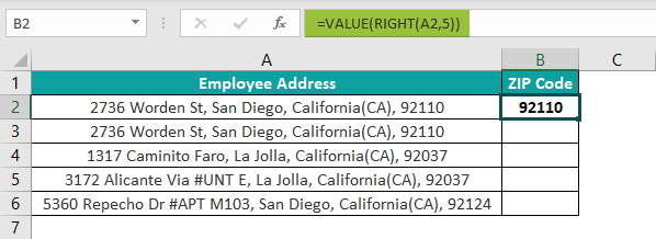
Step 2: Drag the fill handle downwards to copy the formula in cell range B2:B6.

In the above formula, the RIGHT() extracts the ZIP Code from each text string in column A. And the VALUE() converts the ZIP Codes into proper number format.
Likewise, we can use RIGHT() with VALUE() in Excel.
Example #4
Here we shall see how to use the RIGHT function in Excel to extract a substring that appears after a specific character in a text string.
Suppose the students’ full names in the table below are the text strings from which we need to get the last names.
So the character we need to track is the blank space between the first and last names in each cell to extract the last name using the RIGHT().
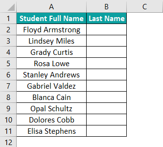
In such scenarios, we need to use the RIGHT() with LEN() and SEARCH() to achieve the required output.
Step 1: Select cell B2, enter the below formula containing RIGHT(), LEN(), and SEARCH(), and press Enter.
=RIGHT(A2,LEN(A2)-SEARCH(” “,A2))
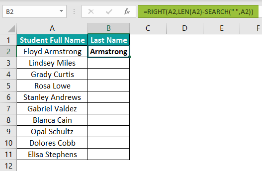
Step 2: Drag the fill handle downwards to copy the formula in the range B3:B11.
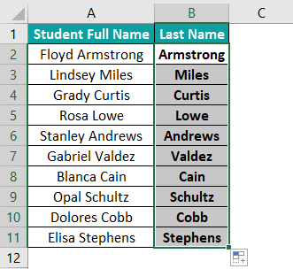
The SEARCH() finds the blank between the first and last name in each text string in column A. The difference between the LEN() and SEARCH() chooses the last name, and the RIGHT() returns the selected portion of the full name.
The three functions ensure we do not have to enter a unique RIGHT() formula in each cell, though the last names are of different lengths.
Example #5
In this example, we shall use the RIGHT function in Excel to extract a substring after the last appearance of the delimiter in a text string.
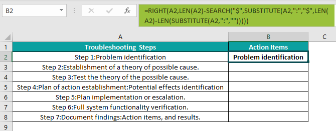
Suppose the below table contains the source data in column A and the delimiter in this case is ‘:’.

Here is how we can extract the substring following the last appearance of the delimiter, ‘:’.
Step 1: Select cell B2, enter the formula containing the RIGHT(), LEN(), SEARCH(), and SUBSTITUTE() provided in the Formula Bar in the below image, and press Enter.
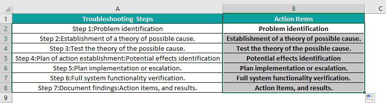
Step 2: Drag the fill handle downwards to copy the formula in range B3:B8.
In the above example, the LEN() containing the SUBSTITUTE() detects the ‘:‘ in the entire text string. And the SUBSTITUTE() replaces the last delimiter with a specific character i.e., ‘$’.
Then, the SEARCH() determines the last delimiter position in the text string, which we replaced with a specific character. Since the character we use for replacement is case-insensitive, the SEARCH() will work.
Otherwise, we have to use FIND(). So, these functions determine the second argument, num_chars.
Likewise, the RIGHT() displays the chosen text based on the number of characters calculated as the second argument.
Important Things To Note
- The RIGHT function in Excel is useful for formatting text and extracting text appearing after a certain character.
- The RIGHT() always returns text characters as the output.
- While the default value of num_chars is 1, if it is more than the text string length, the RIGHT() will return the entire text string.
- The num_chars argument value which is less than zero results in the RIGHT() returning the #VALUE! error.
- If we want the RIGHT() to return a number in the correct format, we should use it with the VALUE().

Frequently Asked Questions (FAQs)
There is a RIGHT function in Excel in the Formulas tab. We can select the target cell and click on Formulas > Text > RIGHT to access the function.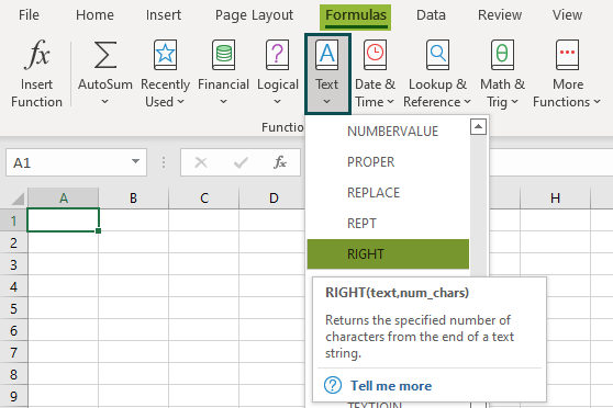
Once we click on the RIGHT(), the Function Arguments window opens, where we need to enter the arguments’ values to execute the formula.
Alternatively, we can select the target cell and enter the RIGHT() after the ‘=‘ symbol, with the required arguments’ values.
The RIGHT function may not work due to the following reasons:
1. The source text string might contain one or more trailing spaces.
2. The num_chars argument is a value below zero.
3. The source text string is a date.
We can obtain results using LEFT and RIGHT functions in Excel with a few steps.
Let us see the steps using an example.
Suppose we need to remove the trailing slash in the below URLs of column A and display the updated URLs in column B.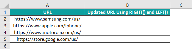
We can use the functions LEFT and RIGHT together to achieve the required result. The steps are:
Step 1: Select cell B2, enter the below formula containing RIGHT() and LEFT(), and press Enter.
=LEFT(A2,LEN(A2)-(RIGHT(A2)=”/”))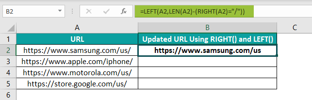
Step 2: Drag the fill handle downwards to copy the formula in range B3:B5.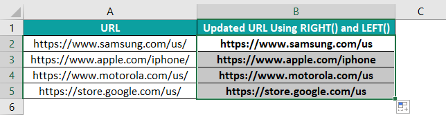
Here, the RIGHT() will take the default value of 1 for the second argument, num_chars. Thus, it returns ‘/’.
So, the RIGHT() return value will be equal to “/”, which makes the condition true or 1. The LEN() counts the total source text string length in the specific cell.
Thus the second argument in the LEFT() will be one less than the total text string length. And so, the LEFT() displays the entire text string leaving the last character in the text, ‘/’.
Download Template
📥Download the ready-to-use Excel template to practice this tutorial yourself.
RIGHT Function In ExcelRecommended Articles
This has been a guide to Right Function in excel. Here we discuss how to use RIGHT function & formula with examples and downloadable excel template. You can learn more from the following articles –
Leave a Reply