
What Is VLOOKUP Using Names In Google Sheets?
The VLOOKUP Names in Google Sheets is a VLOOKUP function with its range argument value specified as a named range of cells.
Users can apply the VLOOKUP Names in Google Sheets when they need to use the same lookup range in different VLOOKUP functions across one or more sheets. Also, using names in the VLOOKUP functions makes them more straightforward to apply.
Use this VLOOKUP Names In Google Sheet Template to follow along with the examples in this article.
Download Excel TemplateFor example, the source dataset contains a store’s monthly inventory level data and whether the monthly inventory capacity limit is reached for each month.

We must find the inventory level and whether the monthly inventory capacity limit is met for the month cited in cell F1. We shall consider cells F3 and F4 as the target cells.
Then, we can implement the VLOOKUP(), which works like the Excel VLOOKUP function, with its range argument value being a named range, in the target cell to fetch the anticipated outcome. The logic is based on the meaning of VLOOKUP Names In Google Sheets explained above.

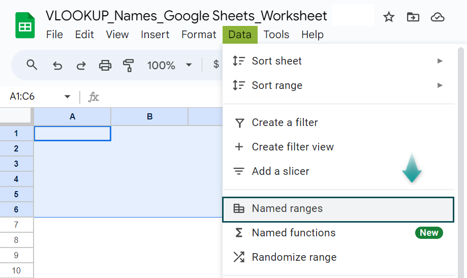
First, we will select the lookup range A2:C13, where we want the VLOOKUP() to look for the search key. Next, choose the Named ranges option under the Data tab to open the Named ranges pane on the right of the workspace.
Next, please enter the phrase we want as the name for the chosen range in the first field in the Named ranges pane, while the second field shows the chosen range address. Click Done.
After that, select the target cell F3 and enter the VLOOKUP(). The first argument is cell reference F1, containing the specified month, Aug, followed by a comma. Next, when entering the range argument, type M or Mo. We shall see the list of functions and named ranges starting with the typed characters, including the one we created. Click the required named range to choose it, and enter a comma. After that, since we require the inventory level value, the third argument, index, value will be 2. The reason is that the required data is in the second column from the first column of the lookup named range. Next, since we are looking for an exact match for the search key in the named range, the last argument, is_sorted, will be 0.
Finally, close the bracket and press Enter to execute the formula.
Thus, the formula VLOOKUP Names in Google Sheets returns 2000 as the required inventory level value for the specified month.
Likewise, the formula remains the same in the next target cell F4. However, the index argument value will be 3. The reason is that we need the status indicating whether the inventory capacity limit has been reached for the cited month. And, it is the third column from the first column of the lookup named range.
Thus, in this case, the formula VLOOKUP Names in Google Sheets returns Yes as the required status for the specified month.
Key Takeaways
- The VLOOKUP Names in Google Sheetsis a VLOOKUP() where the specified range argument value is a valid named range defined in the active Google Sheets document.
- The VLOOKUP functions with named ranges in Google Sheets are helpful since we can create a dropdown list of named ranges representing different lookup tables. Then, we can switch between the named ranges to quickly choose the required lookup table for the concerned VLOOKUP function.
- We must ensure that we follow the naming convention rules while naming a specific cell range using the Named ranges option in Google Sheets. Otherwise, Google Sheets will not accept the entered name and allow us to proceed.
How To Use VLOOKUP With Named Range In Google Sheets?
Before understanding the steps to use the VLOOKUP() with a named range in Google Sheets, we must know how to create a named range.
- Choose the required cell range.
- Select the Data tab → The Named ranges option.
Otherwise, click the Name box dropdown arrow → the Manage named ranges option.
- The Named ranges window will open on the right of the workspace. We must enter the phrase we wish to name the chosen range with, and the second field will show the chosen range reference.

Please note that if we do not choose a cell range and open the Named ranges pane using the option mentioned in Step 2, the pane will show the + Add a range option. We can click it, enter the required name in the first field and use the icon under the second field to update the required range address.
- Click Done to complete the action and close the Named ranges pane.
Furthermore, we must adhere to the following naming convention when naming the required range:
- The name can include only letters, numbers, and underscores.
- The name cannot begin with a number or the phrases “true” or “false”.
- The name cannot include any spaces or punctuation marks.
- The name can have 1 to 250 characters.
- The name cannot be in the A1 or R1C1 syntax.
Next, the steps to implement the VLOOKUP function with a named range in Google Sheets are as follows:
- Select the cell where we want to showcase the outcome.
- Type =VLOOKUP( in the cell. [Alternatively, type =V or =VL and click the function name VLOOKUP from the listed suggestions to choose it.]
- The VLOOKUP() syntax is:

Where,
- search_key: The value to look for in the first column of the lookup array.
- range: The top and bottom bounds of the lookup cell range.
- index: The index of the column in the cited range that holds the return value, and it is a positive number.
- is_sorted: The value representing if the VLOOKUP() must find an exact or approximate match.
- FALSE (0): The recommended value denoting an exact match search.
- TRUE (1): It denotes an approximate match search, with the function considering it as the default value when we omit the argument.
Also, for an approximate match, the search value range must be sorted in ascending order. Otherwise, the function output may be an error.
So, enter the first argument, search_key, and enter a comma. Next, we must supply the range argument. For that, type the starting characters of the named range we created to view all the functions and named ranges starting with the specified characters. Click the required named range in the listed options to choose it and enter a comma. Finally, enter the last two arguments, index and is_sorted, of the VLOOKUP(), separated by a comma, and close the bracket.
- Press Enter to fetch the formula output.
Examples
Let us see the practical methods of using the VLOOKUP() with named ranges, emphasizing the meaning of VLOOKUP Names in Google Sheets explained previously.
Example #1
The first dataset contains the order codes and their order data. The second dataset lists the order codes and the order delivery status.

The aim is to update the order delivery status for each code in the first dataset based on the data provided in the second dataset. We shall consider cells D2:D11 as the target cells.
Then, we can perform the evaluation mentioned above using VLOOKUP Names in Google Sheets, as explained below.
- Step 1: Choose the cell range F2:G11 and then Data → Named ranges.

The Named ranges pane opens on the right end of the window.

- Step 2: Update the first field in the pane with the phrase we want as the name for the chosen range. Also, the second field will show the chosen cell range address.

Click Done to view the newly-created named range details in the Named ranges pane, as depicted below.

Close the Named ranges pane.
- Step 3: Select the first target cell D2 and enter the VLOOKUP().
=VLOOKUP(

The first argument is the cell reference A2, containing the first code in the dataset. Next, enter a comma.

Next, the lookup range is F2:G11, which we have named as OrderCode_DeliveryStatus.
So, type “O” to view all the functions and named ranges starting with the character “O”. We see the named range we created at the bottom of the list.

Click the required named range to update it as the range argument in the VLOOKUP(), and enter a comma.


After that, enter the index argument value as 2 since we require the order delivery status, which is the second column from the search key range in the lookup named range.
Next, enter a comma.

After that, update the last argument, is_sorted, value as 0 since we need the VLOOKUP() to perform an exact match, and close the bracket.

- Step 4: Press Enter to execute the formula in the first target cell.

- Step 5: Use the fill handle option to feed the formula into the remaining target cell.

The formula in all the target cells remains the same, with only the first argument value changing with the order code.
We shall check the cell D11 formula to understand the logic.
The VLOOKUP() looks for the order code TSS_20 in the first column of the named range F2:G11. It finds a match in cell F11. So, it returns the value in the cell where row 11 and column G meet, as the supplied index argument value is 2, which is the cell G11 value of “Cancelled”.
Example #2
Let us see an example of VLOOKUP Names in Google Sheets from another sheet.
The first dataset is in the first sheet. It shows a list of employees and their IDs.

The second sheet contains two sets of data. The first set holds the employee IDs and their designations. The second contains the employee IDs and their contact numbers.

We must update the employees’ designations and contact numbers in the first dataset based on the data provided in the second sheet. We shall take the range C2:D7 as the target cells.
Then, here is how to fetch the target data using VLOOKUP Names in Google Sheets.
- Step 1: Choose the cell range A2:B7 in the second sheet and then Data → Named ranges.

- Step 2: Once the Named ranges window opens, update the required name in the first field for the chosen cell range, with the selected range address showing in the second field.
Click Done.

- Step 3: Choose the range D2:E7 and click the + Add a range option in the Named ranges pane.

Next, iterate Step 2 to name the chosen range.

Click Done and close the Named ranges pane.
- Step 4: Choose cell C2 in the first sheet, enter the VLOOKUP(), and press Enter.
=VLOOKUP(B2,EmpID_Designation,2,0)

Next, utilizing the fill handle, implement the formula in the range C3:C7.

- Step 5: Choose cell D2, enter the VLOOKUP(), and press Enter.
=VLOOKUP(B2,EmpID_Contact_No,2,0)

Next, utilizing the fill handle, feed the formula in the range D3:D7.

So, this VLOOKUP Names in Google Sheets from another sheet example shows that once we set a named range in a Google Sheets file, we can directly use it in any sheet in the file. We do not need to provide the complete address of the range, which might be tedious otherwise.
Furthermore, the VLOOKUP() logic remains the same, even when referring to the named ranges in one sheet from another sheet.
Example #3
We have two datasets. While the first one shows the quarterly sales data of Firm_A, the second contains the quarterly units sold data for Firm_B.

Consider that we must show the quarterly data for the quarter cited in cell G2, based on the specified firm in cell H2. Assume we must show the target data in column I cells.
Then the method is as follows:
- Step 1: Select the range A2:B6 and then Data → Named ranges.

- Step 2: The Named ranges pane will appear, where we update the chosen range’s name in the first field, while the second field displays the selected range address. Click Done.

- Step 3: Choose the cell range D2:E6 and click the + Add a range option in the Named ranges window.

Update the selected range’s name in the first field while the second field displays the selected range address. Click Done.


So now, we have two named ranges, Firm_A and Firm_B.
- Step 4: Select cell H2 and then Data → Data validation.

The Data validation rules pane will appear.

Click the + Add rule option, which will show the fields to update to view a dropdown list in the chosen cell.
The select cell address appears in the first field. Next, since we require a dropdown list in the chosen cell, set the criteria field as the Dropdown option.
After that, update the named ranges names in the next two fields to show them in the dropdown list.
Click Done and close the pane.


Now, we shall see a dropdown button in the chosen cell H2, clicking which we can view the two named ranges.

- Step 5: Choose cell I1, enter the VLOOKUP() containing the INDIRECT(), which works as the Excel INDIRECT function, as its range argument value, and press Enter.
=VLOOKUP(G1,INDIRECT(H2),2,0)

- Step 6: Choose cell I2, enter the VLOOKUP() containing the INDIRECT() as its range argument value, and press Enter.
=VLOOKUP(G2,INDIRECT(H2),2,0)

- Step 7: Click the cell H2 dropdown button and select Firm_A from the list.

Cells I1 and I2 will show the required quarterly data for the chosen firm.

Similarly, we can do the same for Firm_B.


Next, when we change the quarter in cell G2, the output changes accordingly.

First, the INDIRECT() returns a reference to the named range specified in cell H2. Next, the VLOOKUP() searches for an exact match for the search key value in the corresponding named range. Accordingly, it returns the return value from the column the index argument indicates in the specified named range as the output in the target cell.
Important Things To Note
- The VLOOKUP function and the named range in a VLOOKUP Names in Google Sheets formula are not case sensitive.
- When the VLOOKUP function in Google Sheets does not find a match for the search key value in the supplied named lookup range, the function output is the #N/A! error value.
- When the named range supplied as the range argument value to the VLOOKUP() does not exist in the specific Google Sheets document, the function returns the #NAME? error.
Frequently Asked Questions (FAQs)
We can use wildcard characters with VLOOKUP Names in Google Sheets, as explained below with an illustration.
The source dataset lists unique product IDs and their total costs.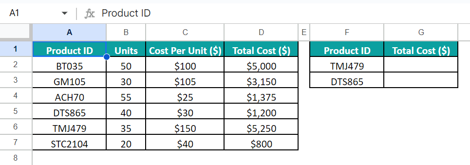
The requirement is to update the total costs of the product IDs listed in column F and show the output in the corresponding column G cells.
Then, we can use the wildcard character, ‘*’, in the VLOOKUP() with a named range to apply the formulas in the two target cells quickly.
• Step 1: Select the range A2:D7 and then Data → Named ranges.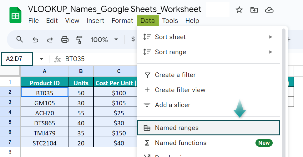
• Step 2: The Named ranges pane will pop open, where we will update the required name for the chosen cell range in the first field, with the second field showing the chosen range address. Next, click Done.
• Step 3: Select cell G2, enter the VLOOKUP(), and press Enter.
=VLOOKUP(“T*”,Product_Data,4,0)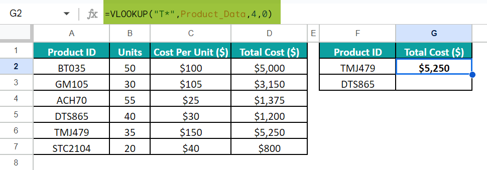
• Step 4: Select cell G3, enter the VLOOKUP(), and press Enter.
=VLOOKUP(“D*”,Product_Data,4,0)
Each product ID listed in the named range starts with a different character. So, when we supply the search_key argument value to the VLOOKUP(), we can enter the first character of the specific product ID, followed by the wildcard character ‘*’, in double quotations.
Next, the VLOOKUP() looks for an exact match for the product ID starting with the character cited before the ‘*’ character in the named range specified as the range argument value. The ‘*’ character represents the characters after the first character in the product ID.
Next, since the total cost values are in the fourth column from the first column in the named range, the index argument value is 4. Accordingly, the function’s output is the return value in the corresponding row (where it finds the match) of the column the index argument value indicates.
The main benefits of using named ranges in VLOOKUP in Google Sheets are the following:
• We can utilize the same VLOOKUP formula across the different sheets.
• We can toggle between lookup tables with a dropdown list or menu.
The VLOOKUP Names is not working in Google Sheets because of the following reasons:
• The VLOOKUP function does not find a match for the search key value in the named range and returns the #N/A error.
• The named range supplied as the range argument to the VLOOKUP function does not exist in the current file.
• The range containing the return value is on the left of the search key range in the named range.
Use this VLOOKUP Names In Google Sheet Template to follow along with the examples in this article.
Download Excel TemplateRecommended Articles
Continue with these related resources when you want the next practical step in this topic.
- LOOKUP in Google Sheets
- HLOOKUP In Google Sheets
- VLOOKUP Table Array In Google Sheets
- VLOOKUP True In Google Sheets
- INDEX MATCH Function In Google Sheets
Explore the full Google Sheets Lookup Functions guide or browse Google Sheets Resources.