What Is Fill Down In Excel?
Fill Down is a function in Microsoft Excel that allows for the quick and efficient copying of data or formulas from one cell to multiple adjacent cells within a selected range. This feature saves time and effort by eliminating the need to manually enter the same content repeatedly.
By selecting a cell containing the desired data or formula and then dragging the fill handle to a small square located in the bottom-right corner of the selected cell, Excel will automatically populate adjacent cells with the same content, taking into account any relative references.
📥Download the ready-to-use Excel template to practice this tutorial yourself.
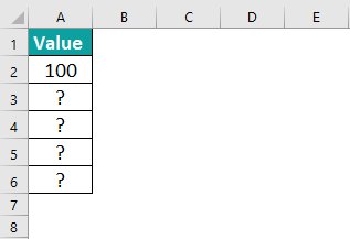
Excel Fill DownThe following example illustrates the usage of the Fill Down function. Begin by positioning the cursor on the empty cell.
Next, press the shortcut key CTRL + D to fill all the cells. To do this, select the cell above and continue selecting cells until reaching the last cell of the data.
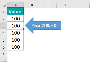
Excel Fill Down Shortcut
The Excel Fill Down shortcut is an efficient and time-saving feature that allows professionals to copy and fill content in a column quickly. By selecting the cell with the desired value and using the CTRL + D shortcut, users can automatically populate adjacent cells with that same value or formula. This function is particularly useful when working with large datasets or generating reports, as it eliminates the need for manual copying and pasting. Moreover, Excel’s intelligent autofill algorithm can recognize patterns and adjust values accordingly, bringing further convenience to data entry tasks. The Fill Down shortcut not only simplifies workflows but also ensures accuracy and consistency in data representation, making it an essential tool for professionals seeking to enhance their productivity and efficiency in Microsoft Excel.
Table of contents
Key Takeaways
- Excel Fill Down is a powerful functionality that enables professionals to manipulate and organize large datasets efficiently while maintaining accuracy and consistency throughout complex calculations or repetitive data entry processes.
- Whether it’s duplicating values, creating sequential number series, copying formulas referencing fixed ranges or cells, or any other specific patterns required, Fill Down offers a versatile solution for streamlining spreadsheet tasks.
- The formula method is a straightforward and user-friendly approach. Users can easily implement, and it does not require any prior knowledge of Power Query or VBA.
How To Use Fill Down In Excel? (With Steps)
To use the Fill Down feature in Excel, professionals can follow a simple set of steps.
- Firstly, select the cell that contains the data we want to fill down.
- Next, locate and click the Fill handle in Excel, a small square in the bottom right corner of the selected cell.
- Dragging this handle downwards expands our selection to include the desired range.
- Alternatively, one can double-click on the Fill handle to automatically fill down until it reaches an adjacent column with data.
- Another option is to use the excel keyboard shortcut CTRL+D after selecting a range of cells or CTRL+R for filling towards the right side instead.
- Moreover, if we need to apply specific formatting to the filled cells or adjust options such as series auto-fill, we can find these settings by opening the “AutoFill Options” button located next to our filled range.
By utilizing these techniques correctly, professionals can efficiently duplicate and replicate formulas or values across multiple cells without repetitive manual input.
Examples
Example #1 – Fill Blank Cells With Above Cell Value
Please consider the following example data for illustration purposes.
To apply this logic, please follow the steps outlined below:

Step 1: Begin by selecting all the cells within the data range.
Step 2: Press the F5 key, which will prompt the appearance of a Go To window.
Step 3: Within the Go To window, click on Special.

Step 4: In the subsequent Go To Special window, choose the option for Blanks.
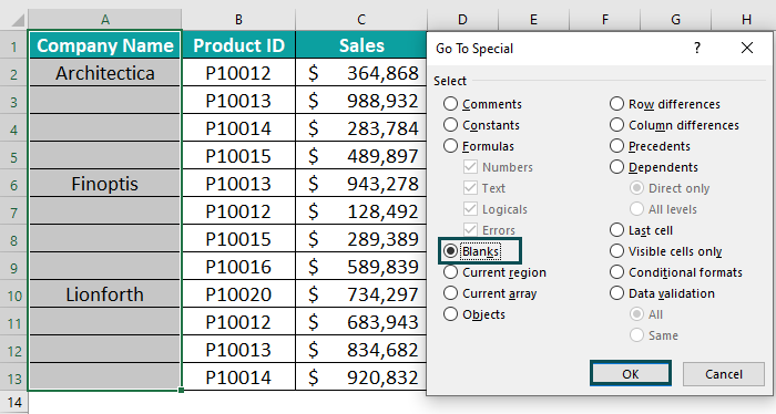
Step 5: This action will select all the blank cells within the designated area.
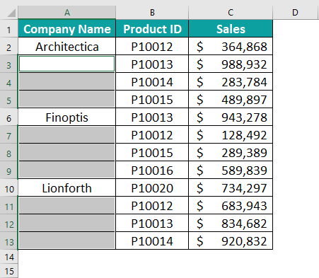
Step 6: Instead of moving the cursor to select any cells, input an equals sign and link it to the cell above.
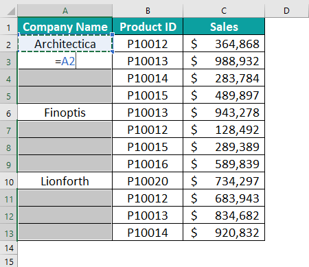
Step 7: After establishing the link to the above cell, refrain from simply pressing the Enter key. Employing a different approach here will prove beneficial; instead, hold down the CTRL key and press ENTER.
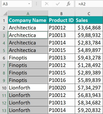
Example #2
The following example explains the use of the Power Query feature in the Fill Down function.
Step 1: To access this feature, the data should be in table format.

Step 2: Navigate to the Data or Power Query tab and select From Table/Range from anywhere within the table. Additionally, we have the flexibility to create a query that connects to a different data source, such as a database or the web.
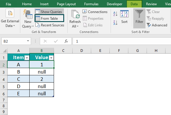
Step 3: Upon selecting this option, the Power Query Editor will open, allowing you to manipulate your data effectively. In Power Query, any empty cells are denoted as null in each respective cell.

Step 4: To fill down the blank cells, you can easily accomplish this by right-clicking on the column header and selecting Fill followed by Down.
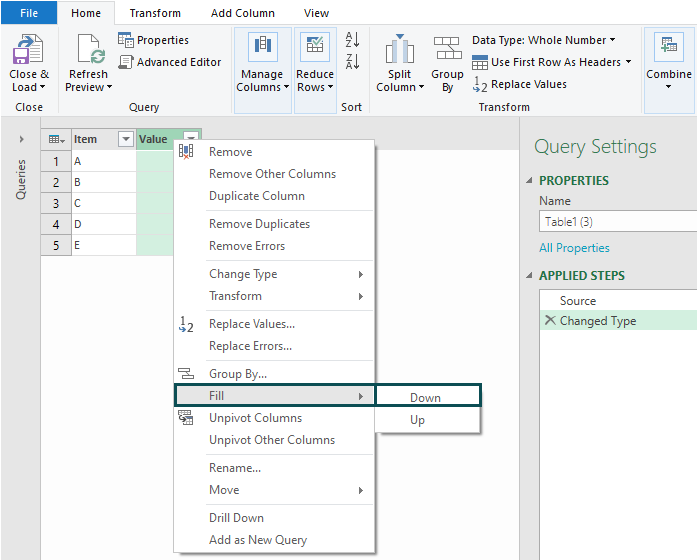
Step 5: By employing the power of Power Query, each section of blank cells within the column will be populated with the value from the cell directly above it.

Example #3
Please consider the following example data provided below for illustrative purposes.
To apply this logic, please follow the steps outlined below:
Step 1: Begin by selecting all the cells within the designated data range.

Step 2: Press the F5 key, which will prompt the appearance of a Go To window.
Step 3: Within the Go To window, click on the Special option.

Step 4: In the subsequent Go To Special window, choose the Blanks option.

Step 5: This action will select all the blank cells within the designated area.
Step 6: Instead of manually selecting cells, input an equals sign and link it to the cell above.

Step 7: After establishing the link to the above cell, refrain from simply pressing the Enter key. Employing a different approach here will prove beneficial; instead, hold down the CTRL key and press ENTER.

Important Things To Note
- The shortcut Ctrl + D is specifically designed to fill down in a worksheet. It cannot fill to the right or left.
- On the other hand, the shortcut Ctrl + Enter is a powerful tool that allows us to fill values into all the selected cells within the worksheet.
- There is another useful feature called the “FILL HANDLE.” This feature also fills down, eliminating the need to drag the formula manually.
- To efficiently fill down, it is recommended to use the Ctrl + D shortcut. Similarly, for filling right, the Ctrl + R shortcut should be utilized.

Frequently Asked Questions (FAQs)
• One limitation is that the fill-down feature only works for adjacent cells in a column or row. If there are blank cells or non-adjacent cells within the range, the feature will not work as expected.
• Additionally, one should be cautious when using this feature with formulas. While Excel automatically adjusts cell references when copying formulas vertically or horizontally, it may not always produce the desired outcome due to relative or absolute references. It is crucial to double-check formula references and ensure they are copied correctly before filling down.
• Use the “Undo” feature, which allows us to revert our actions and return the data to its previous state. This can typically be accessed through a keyboard shortcut (such as Ctrl + Z) or by selecting the “Undo” option from the Edit menu.
• Another approach is to select and delete the affected cells or rows manually. This can be done by either pressing the Delete key on our keyboard or using the Delete option in the right-click context menu.
To illustrate, let us examine the provided sample data below.
Step 1: Now, our objective is to incorporate the “Total” column. Let us first apply a simple formula in cell C2.
Step 2: Enter the formula =A2+B2.
Step 3: By placing the cursor on the bottom right corner of the formula cell, we can utilize the “Fill Handle” feature.
Step 4: Double-click on the “Fill Handle.” Consequently, the current cell’s formula will be automatically populated across all the cells below, saving us valuable time and effort.
Download Template
📥Download the ready-to-use Excel template to practice this tutorial yourself.
Excel Fill DownRecommended Articles
This has been a guide to Excel Fill Down. Here we discuss how to use Fill Down in Excel with examples and downloadable excel template. You can learn more from the following articles –

Leave a Reply