Power Query in Excel

What Is Power Query In Excel?

Power Query in Excel is an add-in introduced by Microsoft in 2013. Power Query is an additional tool that allows users to do various ETL processes. ETL means Extracting the data from multiple sources, Transforming the extracted data to fit in needs of the business reports, and finally Loading the data to either Power BI or Excel.

Power Query is available for both Excel and Power BI. Using Power Query in Excel, we can clean and transform the data, add conditional columns, apply filters to the raw data and get only the required data. After doing the essentials to the data, we can then finally load the data to source systems like Power BI and Excel.

For instance, assume we are bringing the sales data from SQL, which has the data for the last 10 years. However, we need only the last 3 years’ data to analyze, so using a power query, we can apply the date filter as on or after the date and then mention the starting date of the data.

How Do You Enable Power Query?

In Excel 2010 and 2013 Version: Power Query is available from Excel 2013 onwards. However, in the 2010 and 2013 versions of Excel, we need to download the power query from the Microsoft website.

You can click on the following link to download the power query from the Microsoft website.

https://www.microsoft.com/en-us/download/details.aspx?id=39379

When downloading the power query in excel, we need to choose the download version, either 32-bit or 64-bit, as per our Excel bit version.

To enable power query in Excel, we should install it on our computer.

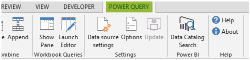
Now we should be able to see the Power Query as a separate tab in Excel.

In Excel 2016, 2019, and Office 365 Versions: In excel versions, Excel 2016, 2019, or Office 365, power query is available under the Data tab in Get and Transform Data group.

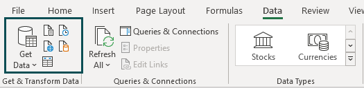
In this group, we have various data sources to insert the data. Then, based on the data source, we can choose any of the above options and launch a power query to perform the ETL process.

Likewise, we can enable power query in Excel.

Power Query Window

Below is the window of the power query editor.

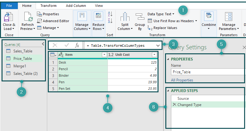
1. Ribbon: It is just like our MS Excel ribbons. Under each ribbon, we have several features to work with.
2. List of Queries: These are the tables imported to excel in this workbook.
3. Formula Bar: It is like our formula bar in excel but here it is M Code.
4. Data Preview: Here, we can see the data preview of the selected query table.
5. Properties: It is the properties of the selected table.
6. Applied Steps: This is an important feature. All the applied steps in the power query are displayed here. We can undo actions by deleting the queries.

What Can You Do With Power Query?

Power Query in excel is an ETL tool for performing various data cleaning and manipulation activities. For example, power Query can do the following activities to assist in data transformation.

• Remove all the unwanted columns.
• Keep duplicate values or remove duplicates.
• Merge two tables into one.
• Append two worksheets or tables of data into one.
• Fill down values from the above cells dynamically.
• Create index columns at various incremental rates.
• Remove error rows.
• Aggregate or pivot the data into summarized rows, thus minimizing the data’s number of rows.
• Transpose of the data.
• Replace values.
• Split the column into first and last names.
• Consolidate multiple workbooks into one.

Likewise, Excel has various kinds of transformation and data clean-up activities.

Examples

Let us look at the following examples to understand power query in excel.

Example #1: Perform VLOOKUP In Power Query

Using power query in excel, we can perform the VLOOKUP operation in the power query by using the merge queries option.

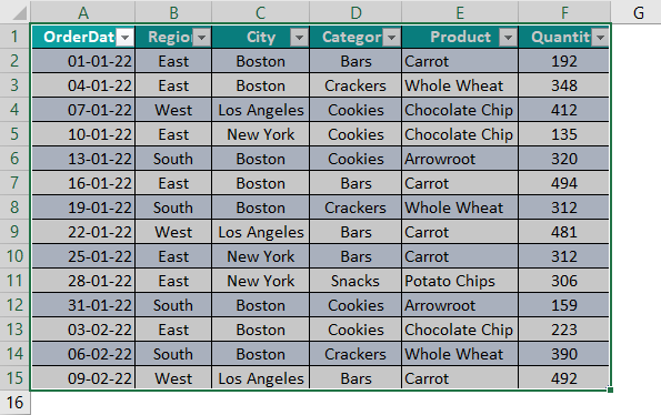
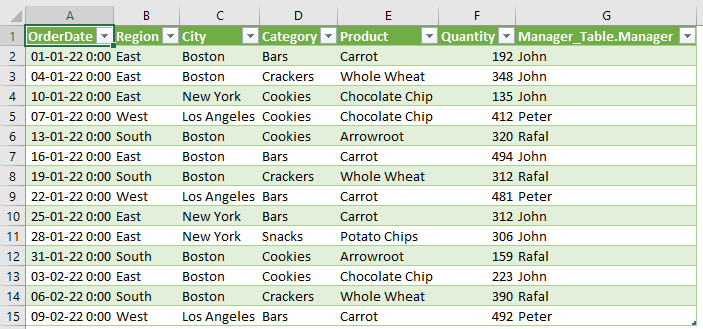
For instance, let us take the following two tables in Excel.

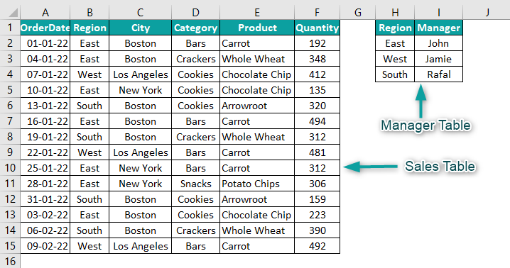
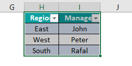
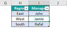
We have a Sales Table and a Manager Table.

Now the objective is to bring add the manager column to the Sales Table by fetching the value from the Manager Table based on the common column between two tables, i.e., the Region column.

The steps used to perform VLOOKUP in power query are as follows:

Step 1: Convert both the tables into Excel Table format. Select any of the cells in the sales table and enter the shortcut keys Ctrl + T. The Create Table window appears.

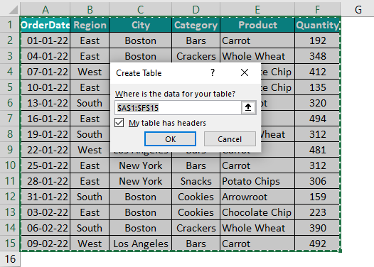
Step 2: Click OK, and the above data will be converted to Excel Table format.

Step 3: Similarly, convert the manager table to Excel Table by performing the above similar steps.

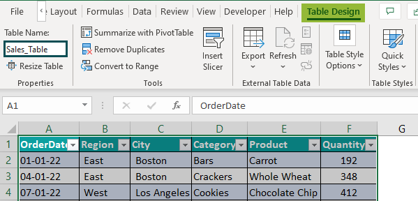
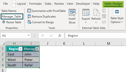
Step 4: Select the sales table. Under the Table Design tab, give the name as Sales_Table.

Step 5: Similarly, give the name for the manager table as well.

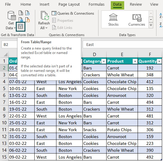
Step 6: Select any of the cells in the Sales_Table. Under the Data tab, click on From Table/Range.

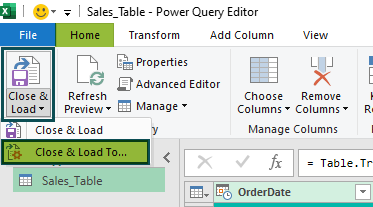
Step 7: The power query editor window opens up. Under the Home tab, choose Close & Load To by clicking on the drop-down list of Close and Load option.

Step 8: The Import Data window pops up. Choose Only Create Connection options.

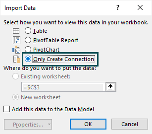
Step 9: Click on OK. Now we can see the new window, Queries & Connections, on the right side of the Excel.

Step 10: Now select the Manager_Table and perform the same steps to create the connection for this table.

Now we can see two connections in the Queries & Connections window.

Step 11: Now, we need to merge these two connections again in the power query.

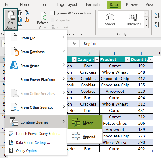
So, go to the Data tab under the Get Data options and choose Combine Queries.

Then, choose Merge.

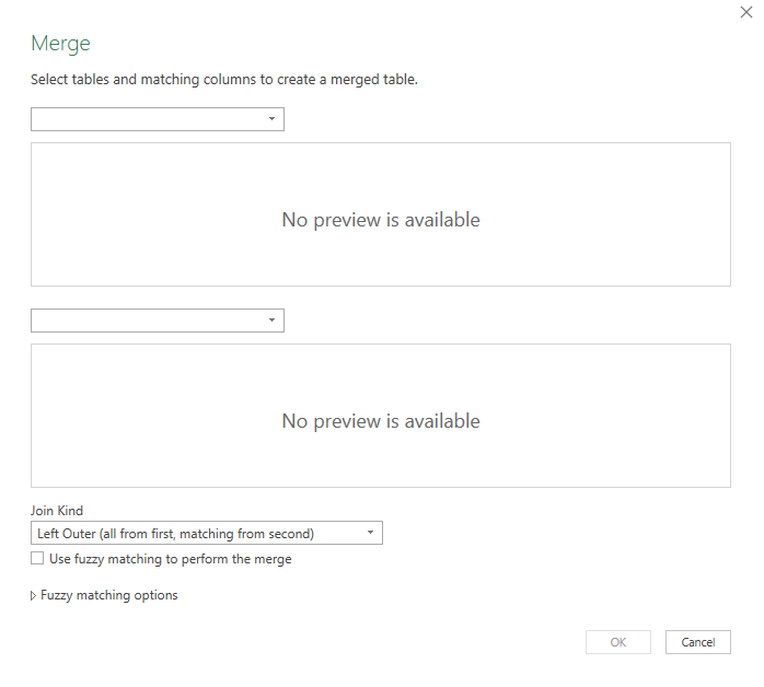
The Merge window pops up, as shown in the following image.

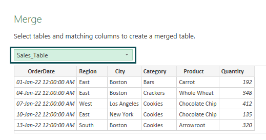
Step 12: Choose Sales_Table in the first drop-down box.

Step 13: Similarly, choose Manager_Table in the second drop-down box.

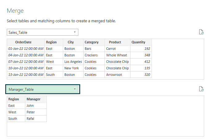
Step 14: Now, choose the common column between the two tables, i.e., Region column in both the tables.

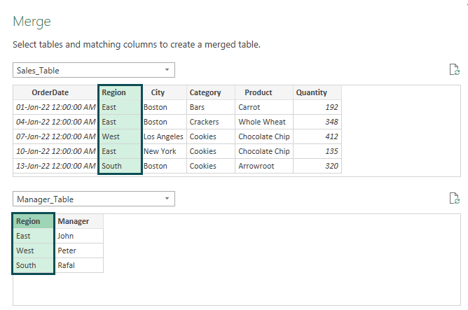
Step 15: In the Join Kind drop-down, choose Left Outer (all from first, matching from second). We can see all the records from the first table (Sales_Table) and matching records from the second table (Manager_Table).

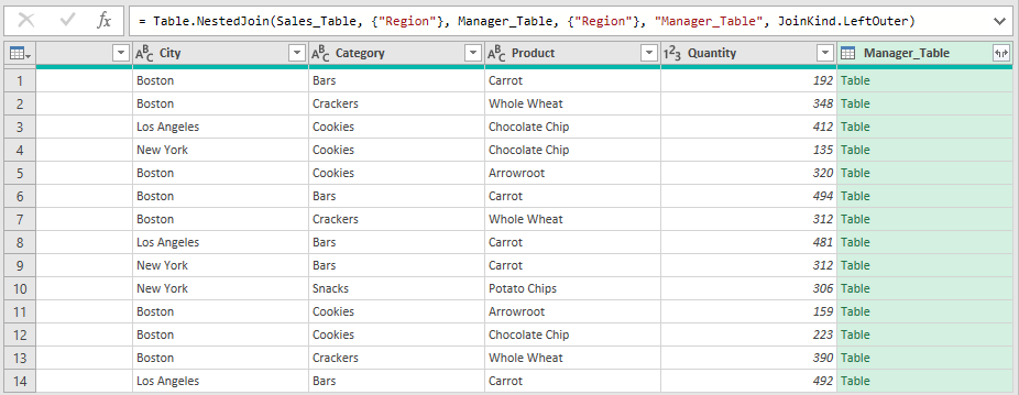
Step 16: Click OK. Once again, the power query editor window appears.

Now, we can see one additional column in the Sales_Table, i.e., Manager_Table.

Step 17: Under the Manager_Table column, click on the double-pointed arrow key.

Step 18: Now, we can see all the columns from the Manager_Table.

Since we only need Manager column, choose only this column.

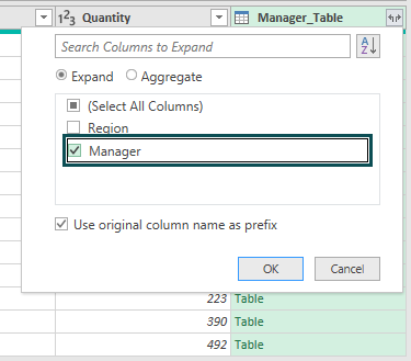
Step 19: Click OK.

We can see the manager column.

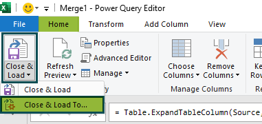
Step 20: Under the Home tab, click on the Close and Load drop-down and choose the Close & Load option.

Step 21: Now, we can see that a new worksheet has been added to the worksheet in the name of Merge1.

This worksheet also shows a newly added column called the Manager column in the Sales_Table.

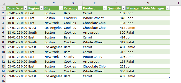
One of the advantages of using power query in excel is whenever the change happens in the Manager_Table; it will dynamically update the results.

For instance, let us change the West manager’s name from Peter to Jamie in the Manager_Table column.

Now in the Queries & Connections window, click on the Refresh icon in the Merge1 query.

Now, queries will automatically update the manager’s name as Jamie.

Example #2: Split Columns Based On Delimiter & Use First Row As Header

Let us use the same data from example #1 but have the data in text or notepad file as shown in the image below:

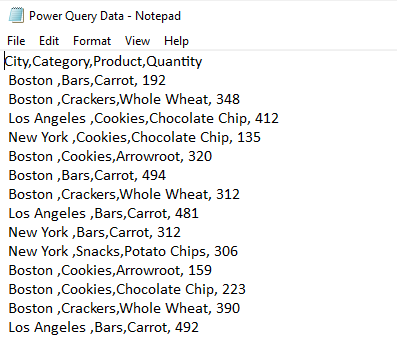
In the above data structure, each column is segregated by a comma. We will try to split columns using power query.

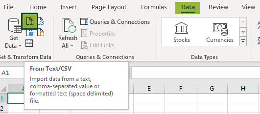
Step 1: Open an Excel file. Under the Data tab, click on From Text/CSV option.

Step 2: Now, excel will ask us to choose the file from the desired folder.

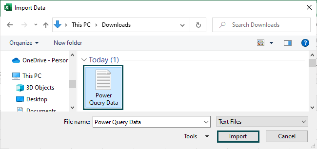
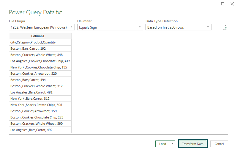
Step 3: Click on Import. Now, we will see the preview of the data.

Next, click on Transform Data.

Step 4: The power query editor window appears, as shown in the image below.

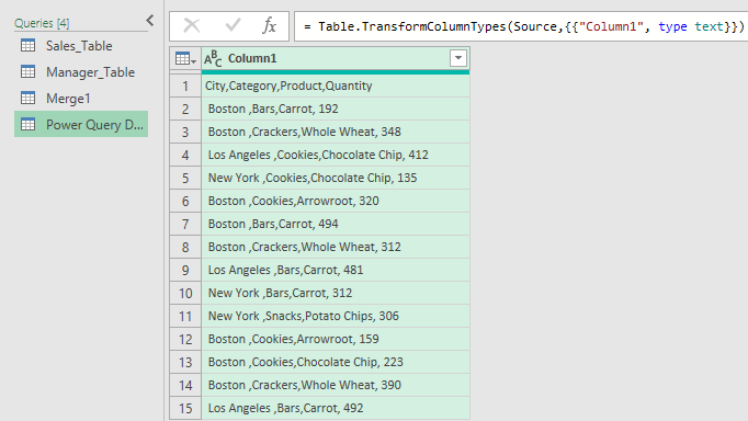
Data is in the desired format. So, let us split the columns.

Step 5: Under the Home tab, we have an option called Split Column. Click on the drop-down list and choose By Delimiter.

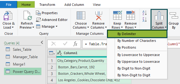
Step 6: In the Split Column by Delimiter window, we need to choose the delimiter separating each column.

In this case, ‘Comma’ is the delimiter separating each column. So, choose a comma as the delimiter.

Step 7: Under the Split at section, choose the option Each occurrence of the delimiter

since we need to separate the column whenever there is a comma, which is the delimiter in our example.

Step 8: Now click on OK. We can see that the data is split into columns.

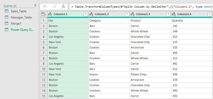
However, the problem here is that power query in excel did not recognize the data headers.

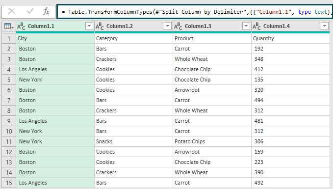
Therefore, we need to do another transformation here. So, we should promote the first row of the data as Headers.

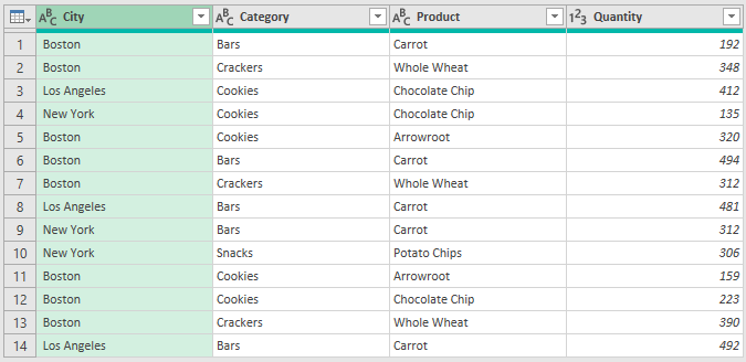
Under the Home tab, click on Use First Row as Headers.

When we click on this option, the data will have the first row as headers.

Example #3: Unpivot Data

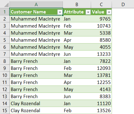
In some cases, the summarized data may appear like the below table.

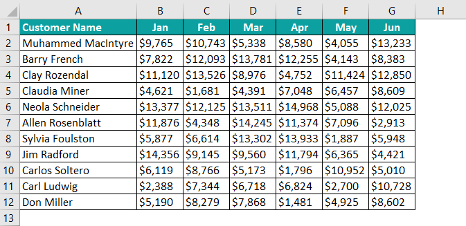
The summarized table shows the monthly sales of each customer. However, for analysis purposes, we need the data to be in tabular format, i.e., each customer data should be in a separate row.

Let us unpivot these columns in the power query.

Step 1: Load the data to the power query.

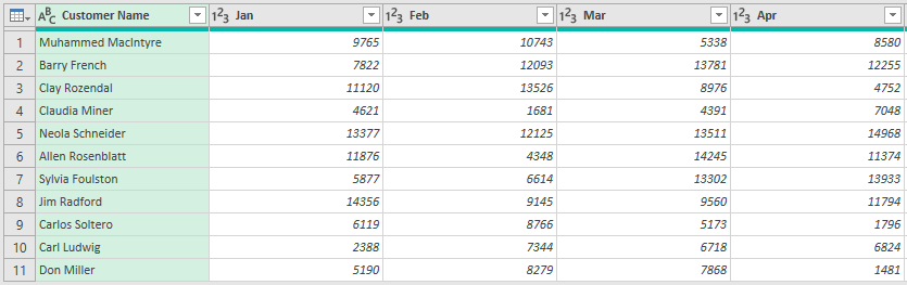
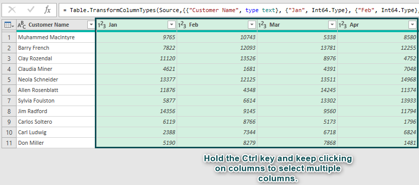
Step 2: Select only the columns we want to unpivot, i.e., select all the month columns.

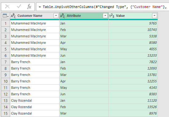
Step 3: Go to the Transform tab and click on Unpivot Columns.

Step 4: As soon as we click on unpivot columns, we can see the transformed data, as shown in the following image.

Step 5: Click on Close and Load under the Home tab.

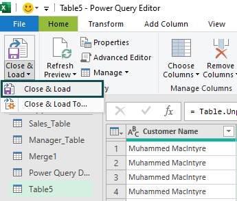
Now the unpivoted data gets loaded to the Excel worksheet.

Important Things To Note

• Power Query in excel is an add-in available for the 2010 and 2013 versions. However, from Excel 2016 version onwards, we have a power query embedded in Get and Transform group under the Data tab.
• It always converts the Excel data into Excel Table format.
• The tool uses M code for its formulas making formulas in Power Query in excel different than Excel formulas.
• Power Query M code is case-sensitive and can perform various activities like unpivot columns, insert Index columns, etc.,

Frequently Asked Questions

Download Template

This article must be helpful to understand the Power Query in excel, with its formula and examples. You can download the template here to use it instantly.

Recommended Articles

This has been a guide to Power Query in excel. Here we discuss how to use power query with examples and downloadable excel template. You can learn more form the following articles –

• Pivot Table In Excel
• Pivot Chart In Excel
• Slicers in Excel