
What Are Slicers In Excel?
Filtering the data in Excel using an auto filter is one of Excel’s most commonly used tools. However, Excel introduced a visual filter called Slicer in the 2010 version. Slicers in Excel help us to filter the data from a visual filter for pivot tables, pivot charts, and Excel Table formats. Unlike auto filters, slicers will display the values in their list. However, users must click on the value when filtering from the pivot table or chart.
Once the slicer is selected, we can customize it to change the color, size, and number of columns to show in the slicer, along with many other custom formatting options. For instance, consider the following pivot table showing the pricelist of eatables. But, first, let us understand how slicers in Excel work.

We can see two slicers for columns Region and City, which help us filter the data for the selected region and city. We have filtered the East region from the Region slicer and the ‘New York’ as the City slicer. The pivot table shows the summary for the selected region and city.
Likewise, we can filter data using slicers in Excel.
Use this Slicers in Excel Template to follow along with the examples in this article.
Download Excel TemplateKey Takeaways
- Slicers allow users to filter the data with a visual selection.
- It can filter the other slicer, so the drill-down is dynamic.
- If the slicer is inserted for one pivot table by default, it will filter only that particular pivot table summary. However, by changing the report connections, we can link one slicer to impact multiple pivot tables.
- We cannot hide any items from the slicers.
- Slicer and pivot tables are interdependent. If we filter one value in the pivot table, it will also filter the same value in the slicer.
How To Use/Insert Slicer In Excel?
Now, we know that slicers in excel are used to filter data. So, let us learn how to use slicers in excel with the following example.
Let us consider the following data.
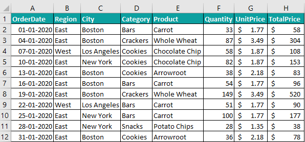
We need to format and convert the above data into an Excel Table using the following steps:
Step 1: Select any of the cells in the data range.
Step 2: Press the Excel table shortcut keys, Ctrl + T.
Step 3: The Create Table window pops up. Enter the data in Where is the data for your table? Box.
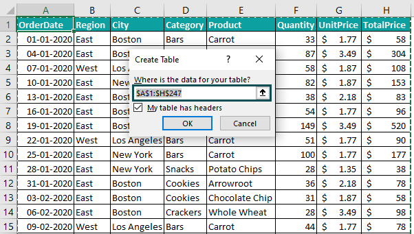
Step 4: Click OK.
We can see that the data is converted into Excel table format.
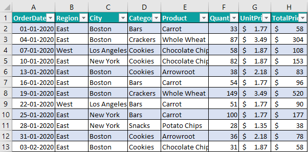
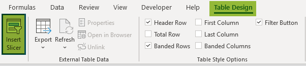
Once the data is converted into Excel table format, the Table Design tab appears in the Excel ribbon.
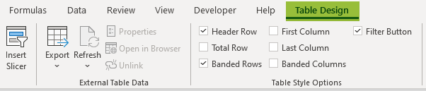
Under the Table Design tab, click on the Insert Slicer option.
The Insert Slicer window with the list of all the available columns in the Excel table pops up.
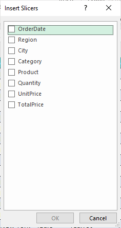
Please select the columns for which we need to insert the slicer.
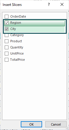
After selecting the desired columns, click OK.
Immediately, we can see slicers for the selected columns.
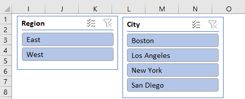
Now click on any of the cities from the city slicer, and the selected city data will be filtered in the Excel table.
Another thing about the slicer is that when we select a particular city, it will filter the other slicer as well, i.e., Region Slicer.

As we can see, we can select only the ‘East’ region from the region slicer, and the other part, ‘West,’ is hidden.
Likewise, we can filter data using slicers in Excel.
Slicer In Excel Examples
Example #1 – Insert Slicers For Pivot Tables
We use slicers when we create a pivot table to summarize the data. So, let us take the same data from the above example to build the pivot table summary report.
Now, we will use the data already converted into Excel table format.
Using the above data, insert a pivot table to show the monthly sales summary, as shown in the following image.
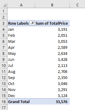
We have the monthly sales summary. After inserting the pivot table, we can insert slicers to slice the data based on the selection we make from the slicer.
Why Slicers: The real question is why we need slicers when we can drag and drop fields to see the summary. For instance, if we want to see the product-wise sales based on month, then we can use the product column in the columns section of the pivot table.

The pivot table has become wide and hard to read. Now, if we need to analyze based on the city, we can include the city column in the pivot table.
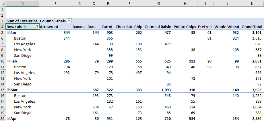
We can see that increase in the number of fields makes it more complex to understand.
So, to avoid the difficulty, we should use slicers to allow the user to slice the data part by part.
To insert a slicer for the pivot table, follow the steps listed here:
Step 1: Select any of the cells in the pivot table area.
Step 2: As soon as we select the cell in the pivot table range, both the Pivot Table Analyze and Design tabs appear in the ribbon.
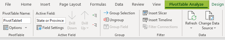
From the pivot table analyze tab, click on the Insert Slicer option.

Step 3: It will bring the insert slicer window with all the dimensions from the table (columns). We can select one or more dimensions to play around with the pivot table.
For instance, only the city slicer will be inserted if we select City.
Similarly, if we select both city and product, we will get the slicers for both columns.
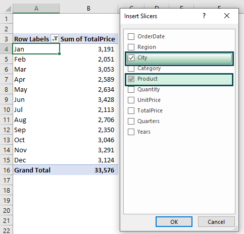
Step 4: Click OK, and we will get a slicer for City and Product columns.
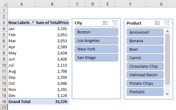
Slicers automatically give only the unique values from both columns and list them in the slicer box.
Working With Slicers
From the inserted slicer, we can filter data. For instance, if we want to see the sales for the produce Carrot, then click on this product in the product slicer.

We can see that only the selected product gets a different color than other products. Now, we can see the monthly sales only for Carrot.
Now, assume we need to get the sales for one city, i.e., New York.
So, select this city from the city slicer.
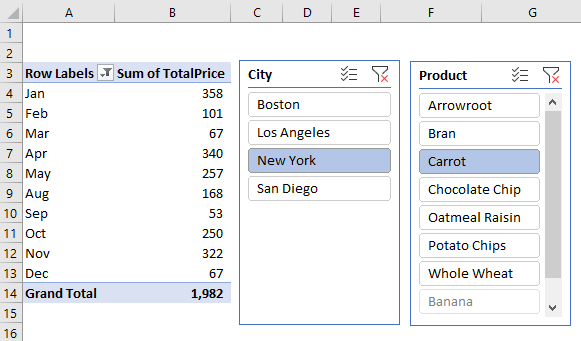
Now, we are seeing monthly sales for Carrot and New York.
If we want to select multiple cities or products, hold the control key and click on the items we want to slice.
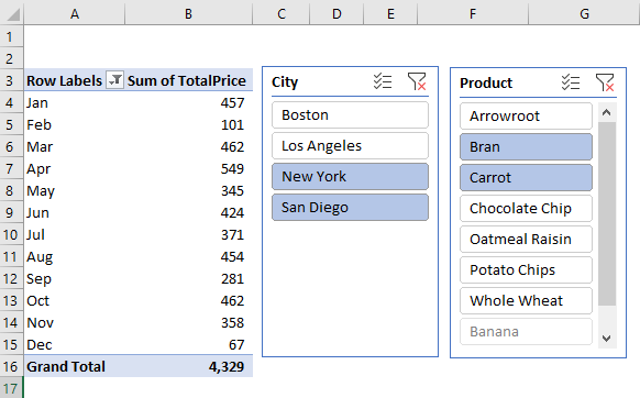
Now we can see the monthly products, Bran and Carrot, for the cities of New York and San Diego.
If we want to remove the slicer selection, click on the filter icon with a red cross mark at the top right corner of the slicer.
Alternatively, we can use the Excel shortcut keys ALT + C to remove selections from the slicer. Select the slicer, hold the alt key, and press the C key.
Example #2 – Link Slicer To Multiple Pivot Tables
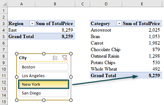
When we want to deal with multiple pivot tables, we may insert slicers for each. For instance, look at the following two pivot tables.
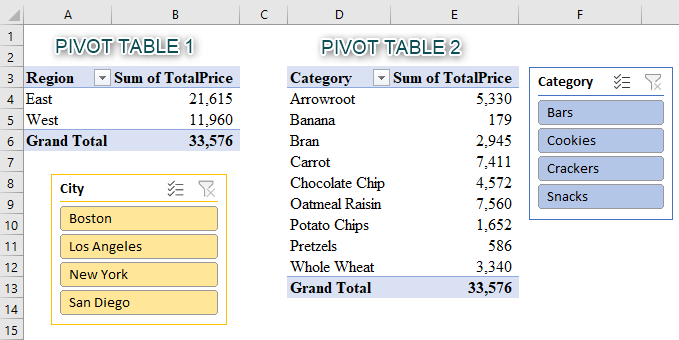
We have two pivot tables, Pivot Table 1 and Pivot Table 2.
For Pivot Table 1, let us add slicers in excel for the city column.
Similarly, for Pivot Table 2, let us add slicers in excel for the Category column.
To check the functionality, let us first select any categories from Pivot Table 1 slicer.
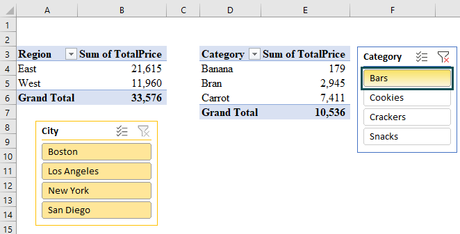
Though we have selected the Bars category, it filtered only Pivot Table 2 and not Pivot Table 1. Similarly, when we select the city from the city slicer, it will filter only Pivot Table 1 and not Pivot Table 2.
Though the two slicers are inserted for two different pivot tables, they do not have any connection with the other pivot table.
When we insert the slicers for two different pivot tables by default, it does not have any connection between pivot tables. Therefore, we need to build a connection between the two tables.
Right-click on the city slicer and click on Report connections… option.
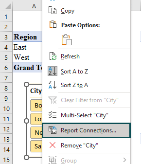
It will connect the slicer’s report with the pivot tables in the Report Connections (City) window.

As we can see, the city slicer only connects with Pivot Table 1, so check the box of Pivot Table 2 to link the city slicer to Pivot Table 2.
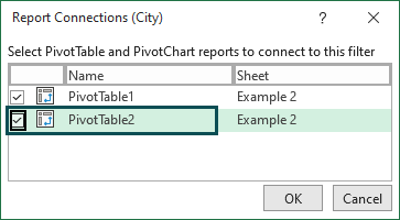
Click OK.
Now, the city slicer can slice Pivot Table 2 as well.
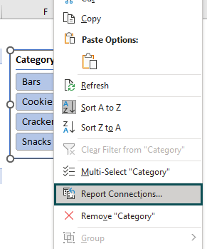
Similarly, we need to build a connection from the Category slicer to Pivot Table 1.
Right-click on the category slicer and click on the Report Connections… option.
Now, link a connection to Pivot Table 1.

Click OK.
Now, both the slicers connect with the pivot tables, and one slicer will filter both tables and slicers.
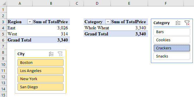
We have selected Crackers from the category slicer, and it has filtered both the pivot tables.
How To Edit Slicer In Excel?
We can edit the slicers to make them look beautiful. But, first, we need to follow the below steps to format the slicer.
1. Remove Header From The Slicer
Adjusting the slicer position in the dashboard is very important because we always end up without having enough space to fit the slicer in the dashboard. In those cases, we can remove the slicer header.
For instance, look at the following slicer.

We have a product header here. To remove it, right-click the slicer and click on Slicer Settings… option.

In the slicer settings window, uncheck the Display Header check box.

Click on OK, and we will no longer see the slicer header.
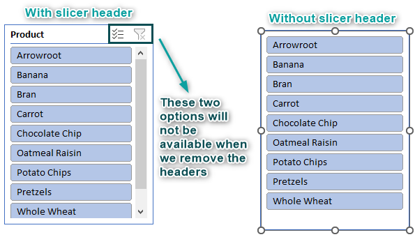
The problem is we cannot clear filters while removing headers.
2. Change Columns And Rows
We will have to scroll down the slicer when many values are filtered. For instance, in the following slicer, we need to scroll down to see other products.
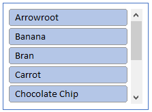
To avoid scrolling down, we can split the data into multiple columns. To do that, select the slicer. Then, the Slicer tab in the Excel ribbon appears.
Under this tab, change the columns to 3.
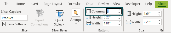
It will change the slicer to 3 columns, and all the rows will be distributed equally.
Now users can easily make the selections without any trouble.
3. Hide Values With No Data In The Slicer Box
When we work with multiple slicers, one slicer filters the other, so some items may not have data when we select one slicer.
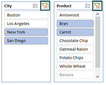
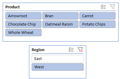
For instance, look at the following two slicers.

We selected ‘West’ and filtered the product slicer in the region slicer. However, not all the products have the data for the ‘West’ region.
As we can see, ‘Banana’ and ‘Pretzels’ are shaded and not allowed to select. So, instead of showing no data, we can hide the items in such situations.
Right-click on the product slicer and click on Slicer Settings… option.

Check the Hide items with no data box in the slicer settings window.

Click OK, and we no longer see items without data.
4. Insert Slicer From Pivot Table Fields
Inserting slicers for the pivot table is done via the PivotTable Analyze tab in the ribbon.
The above method will bring us all the columns from the table. However, if the list of columns is huge, it won’t be easy to find the particular column to insert the slicer.
Instead, we can right-click on the desired column from the pivot table fields and click on Add as a slicer.

Now the selected column will be added as a slicer.
5. Change The Slicer Styles
We can change or design the style of the slicer. Once the slicer is inserted, a new tab called the Slicer appears. It helps us format the slicer.
From the list of available styles, we can choose any one of the styles.
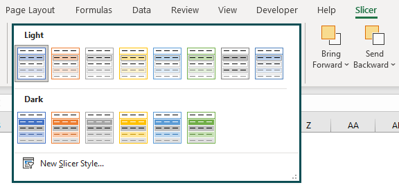
If we want to build a new style, we can click on New Slicer Style… option.
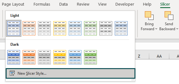
By using this option, we can build a new slicer style.
6. Align The Slicers
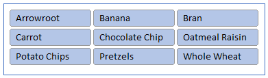
When we insert multiple slicers, it is important to align them to make them look clean and clear. For instance, look at the following image.
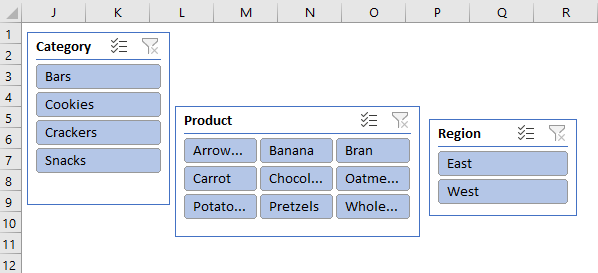
We have three slicers, but they are not aligned properly. To align them properly, select all three slicers using the control key.
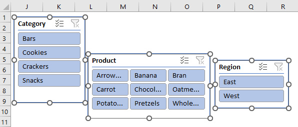
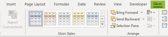
Now go to the Slicer tab under the Arrange category.

It will align all the selected slicers on top.
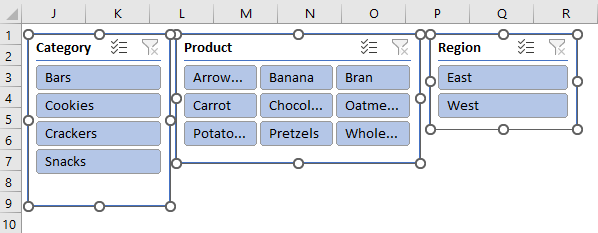
Like this, we can do the alignment of the slicers.
Excel Slicer Not Working
If the slicer is not working, there are two possible reasons.
- File Saved in XLS Format: If the file we are working on in Excel is saved as an XLS file extension, then our slicers might not work properly.
- Excel File in Compatibility Mode: If the Excel file is in compatibility mode, slicers may not work.
Important Things To Note
- Slicers are available from Excel 2010 versions only.
- They can be inserted only when the pivot table is inserted or if the data table is converted to Excel Table format.
- One slicer can contain one column of information only. However, users can modify this to their needs by increasing the number of columns.
- ALT + C are the Excel shortcut keys to remove all the selected values from the slicer. To apply this shortcut key, we first need to select the slicer.
Frequently Asked Questions (FAQs)
Slicers in Excel help filter data in pivot tables and charts.
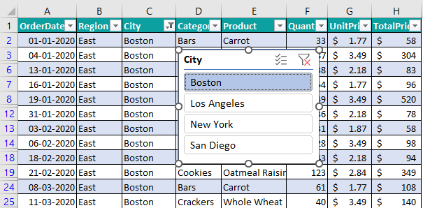
For example, we have the following pivot table in Excel.
The pivot table shows the summary based on the category. Further, we can insert a slicer for the city column to filter the data based on the city.
Go to the PivotTable Analyze tab by selecting any of the cells in the pivot table and clicking on the Insert Slicer option.
It will bring the list of columns with the data set or table. Choose the desired column (City) and then click OK.
Now we have the slicer for the city column.
Click on any city and pivot tables to show the summary only for the selected city.
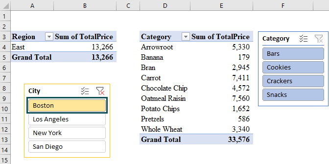
For instance, in the above city slicer, we have selected the city of Boston. As a result, we can see that the pivot table shows numbers only for the city of Boston.
While working with two slicers from two pivot tables, we must create a report connection between pivot tables.
Right-click on the slicer we want to connect and click on the Report Connections… option.
It will show us the list of pivot tables connected and not connected to the slicer.
Check the boxes of the pivot table connections we need to connect.
To lock the slicer, right-click on the slicer and click on Size and Properties.
The Format Slicer window appears on the right side of the Excel screen.
Click on Properties and check the Locked box.
To hide any of the slicers, go to the Home tab. Then, under the Editing group, click on the Find & Select option and select the Selection Pane… option.
We can see the list of slicers we have created in excel.
If we want to hide any slicers, click on the eye icon.
It will hide the Region slicer from the workbook.
Use this Slicers in Excel Template to follow along with the examples in this article.
Download Excel TemplateRecommended Articles
Continue with these related resources when you want the next practical step in this topic.
Explore the full Excel Tables and Data Tools guide or browse Excel Resources.