
What Is Pivot Table In Excel?
Pivot Table in Excel is a tool that allows users to swiftly summarize, analyze and create consolidated summary reports from huge data sets with just a few clicks. It also provides interactivity with the slicers feature.
Pivot Table options help design user-friendly reports, summarizing data in categorical and sub-categorical ways, applying filters, conditional formatting, slicers, subtotals, aggregates numerical data, etc.
Use this Pivot Table In Excel Template to follow along with the examples in this article.
Download Excel TemplatePivot Table in Excel is designed such that not only experts but also beginners can get a summary of the data with just a few clicks. For instance, the table below shows a textile company’s sales data.

By using Pivot Table, we can create a summary report, as shown below.

As we can see in the above image, we have created a summary sales report date-wise and region-wise with nice formatting.
Key Takeaways
- A Pivot Table is used to summarize the data from a large data set interactively.
- Pivot table uses pivot cache to take a snapshot of the data, thus increasing the size of the workbook.
- The Excel Table option makes the data range dynamic for a pivot table. So, whenever we add or delete, we just have to press the refresh shortcut keys ALT + A + R + A.
- Pivot Table helps us to analyze the data with simple drag and drop options. Thus, making it easy to create a consolidated summary of the data.
How To Create A Pivot Table?
Before we create pivot table in Excel, we need to consider organizing the data into rows and columns. Hence, we have created the following sample data to demonstrate pivot table examples.

Before we create pivot table in Excel, we need to organize the data. Whenever we organize the data, we need to keep the below things in mind.
- Always give meaningful heading to the columns.
- Do not have blank rows or columns in the entire data set.
- Make sure no subtotals are present in the data.
Now, we use the below steps to create a pivot table.
- Step 1: Select the entire data range, including headers.

Please Note: Only the selected area will be considered for pivot table calculation purposes. - Step 2: Go to the Insert tab and click on Pivot Table.

- Step 3: The PivotTable from table or range window appears. Here, we can see the range of cells we have selected to create the pivot table.

Please Note: We can also change or readjust the range of cells per the requirement. - Step 4: Next, we need to choose where to place the pivot table. By default, it will prompt for New Worksheet. If we want the pivot table in the same sheet, we need to choose Existing Worksheet.

- Step 5: Click OK. In a few minutes, we will be able to see a new worksheet created separately for the pivot table, as shown in the image below.

Now, let us learn about some of the features of the Pivot Table.
Report Area: In this area, we build our report in the pivot table.
Field Section: These are the fields we use to build reports. These fields are nothing but the columns from the data set that we have selected to create the pivot table.
Layout Area: In this area, we have the following options;
- Rows: This is the area to be used to summarize the data. For instance, if we want to summarize the data based on Ship Mode then we can drag and drop the Ship Mode to the rows. Once we drag and drop the Ship Mode to the rows section, we can see the summarized Ship Mode values in the report area.

- Values: In this section, we will do all our calculations. For instance, if we want to include the sales, then we should drag and drop the Sales column to the Values.

Now we can see total sales based on Ship Mode.
- Columns: After we see the total sales based on Ship Mode, further, we can also drill to another level like Product Category. Drag and drop Product Category to the columns area.

Now we can see total sales based on Ship Mode and Product Category.
- Filters: Further, we can also add some filters to the report we created under the filters section. For instance, if we want to filter based on Region, then drag and drop the Regions column to the filter area.

Likewise, we can create pivot table in excel by using all the above features.
How To Use Pivot Table?
Now, we know how to create a pivot table using features. Next, we will see how to use the pivot table with the same data. Finally, we will try to answer a few questions to know the usage of the pivot table.
What are the Total Sales & Profit for each Customer Segment?
Step 1: Drag and drop Customer Segment to Rows.

Step 2: Now drag and drop the Sales column to the Values section.

Pivot Table has given us the summary of sales based on Customer Segment.
Similarly, drag and drop Profit to the Values section (just below sales) to the Profit summary.

Pivot Table gives us the summary of sales & profit for each customer segment.
What are the top 5 States or Province based on sales?
Step 1: Drag and drop the State or Province column to rows and the Sales column to values. It will give us the total sales based on state.

Step 2: By default, the pivot table alphabetically gives the summary and sorts based on State or Province.
Since we are looking for the top 5 states or provinces, right-click on any of the cells in sales values.

Step 3: Go to Sort and choose Sort Largest to Smallest.

It will sort all the numbers in descending order.

Step 4: Click on the State or Province column’s drop-down list and hover the mouse on Value Filters. Then, choose Top 10.

Step 5: In the Top 10 filter (State or Province) window, enter Top and 5.

Click OK. We will get the top 5 States or Province based on sales as shown below.

Examples
Let us look at a few advanced examples of using a pivot table.
Example 1: Find Profit % Using Calculated Field in Pivot Table
For instance, the below table shows State or Province wise total sales and profit values in the pivot table.

We do not have Profit % in the data; however, by using the pivot table, we can calculate on our own with the following steps:
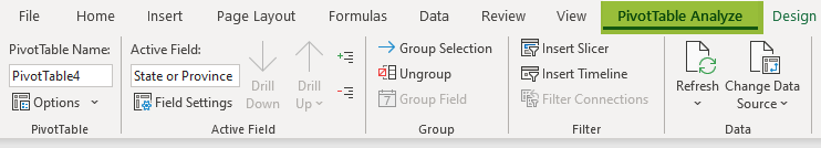
Step 1: Select any of the cells in the pivot table, and click on the Pivot Table Analyze tab.
Step 2: Under this tab, click on the Fields, Items, & Sets drop-down and choose Calculated Field.

Step 3: Next, the Insert Calculated Field window pops up. Give a name for the newly inserted column.

Step 4: In the Formula: box, enter =Profit/Sales, and in the Fields: section, choose Sales as shown in the following image.

Step 5: Select OK. We will be able to see a column as shown below.

As of now, we see zero as the value. It is due to formatting issues.
Step 6: Select the entire column and apply Percentage Formatting.

Likewise, we can create a new calculated column in the pivot table.
Example 2: Grouping Dates in Pivot Table and Number Formatting
Consider the following table showing the sales data of a bakery.

Using this data, we will create a pivot table and understand how to group dates.
Step 1: Select the entire data and press the shortcut keys ALT + D + P + F to insert the pivot table.
Step 2: Drag and drop the Order Date column to rows and the Total Price column to values.

As we can see, we have sales based on each day; but we need to summarize it by Year and Month.
Step 3: Right-click on any of the Order Date columns cells and choose Group.

Step 4: The window named Grouping pops up.

Step 5: Select Years and Months. Click OK.

Click OK. We can see that the data has been categorized into Years and Months.

However, there is another thing we need to do here, i.e., the formatting of numbers.
Step 6: To apply currency formatting for total price, click on the down arrow under the values section and choose Value Field Settings.

Step 7: The formatting window, Value Field Settings pops up. Click on the Number Format option.

Step 8: Under Number Format, select Currency and apply the dollar currency format. Click OK.

Our pivot table will now have number formatting, as shown below.

Example 3: Add Slicers
Please Note: Slicers are available only from Excel 2010 version.
To make the pivot table interactive, we can add slicers.
For instance, if we want to make the pivot table interactive for Product, then select any of the cells in the pivot table and choose Pivot Table Analyze.
Step 1: Click on the Insert Slicer option.

Step 2: In some time, we can see Insert Slicers window listing all the columns where we can choose the desired column.
In this case, let us choose the Product column.

Step 3: Click OK. We can see a slicer, as highlighted in the image below.

From the slicer, we can select any of the products and the pivot table will display a summary for the selected product.

Refresh A Pivot Table
Pivot Table in Excel uses a cache to store the data, and any changes in the source data will not be updated dynamically. So, we need to refresh the data manually. Let us learn how to refresh pivot table in excel using the following example.
For instance, we have added some additional data for the below pivot table.

Ideally, we should select the Pivot Table Analyze tab to refresh the data and click on the refresh button as shown in the following image.

This refresh happens only when there is a change in the existing range of cells. But, if any additional rows or columns are added, it won’t refresh.
To do this, we need to change the range of cells every time. So, click on Change Source Setting and change the source range manually.


However, doing this every time makes the task tedious. So, to make refresh dynamic, we need to convert the data range into an Excel Table.
Select the data range and press Ctrl + T to bring the Excel Table option.

Click OK, and data will be converted to Excel Table format.

Give a name to the Excel table.

Now in the Change PivotTable Data Source window, instead of selecting the table range through the cell, we should give the table name as Sales and click OK.

We just have to click on the Refresh button whenever we make any changes. Or, we can also press the shortcut keys ALT + A + R + A.
Similarly, we can refresh pivot table in Excel.
Move Pivot Table In New Location
We can change the location of the already built Pivot Table.
To change, we need to click on Move Pivot Table under Pivot Table Analyze.

The Move PivotTable window pops up.
In this window, we need to choose where we need to move the pivot table.

If we want to move the pivot table to a new sheet, then choose New Worksheet. To move the pivot table within the same sheet, then choose Existing Worksheet.
Based on our selection, pivot table will be moved to a new location.
Delete A Pivot Table
To delete pivot table in excel, we need to look into below two options.
- If we have a pivot table in the new worksheet without any other data, then we can delete the entire worksheet.
- If the worksheet has some other data, then we need to select the pivot table area and then hit the delete key. To select the entire pivot table quickly, go to Select and click on Entire Pivot Table option from the PivotTable Analyze.

- Using this option, we can select the entire pivot table. Then, press the delete key to remove or delete pivot table in Excel.
Important Things To Note
- The Pivot table in excel is one of the earliest functions introduced by Excel in 1994.
- This table is called ‘Pivot’ as it rotates the rows/columns and presents them from various perspectives.
- Pivot Table uses cache to store the snapshot of the data whenever we create a pivot table in Excel.
- Slicers feature is available only from Excel 2010 and later versions.
- The shortcut keys to create a pivot table are ALT + D + P + F.
- Pivot Table data range should not have any blank columns.
Frequently Asked Questions (FAQs)
Pivot Table in Excel is used to summarize and create consolidated reports from huge data.
The Pivot Table in Excel is under the Insert tab in the Tables group.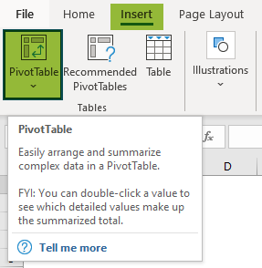
Pivot Table in Excel uses Pivot Cache in the backend. Whenever we insert a pivot table, Excel takes the screenshot of the data and stores it in its memory. Hence, it is called Pivot Cache.
Then, pivot table uses this cached data and starts summarizing the data.
Usually, we use single data range to create pivot table. However, it is possible to create a pivot table with multiple ranges or worksheets as well.
For instance, we have below 4 region-wise sales data.
As we can see, we have the same data structure in all the worksheets.
To include all the worksheets in a single pivot table, press the shortcut keys ALT + D + P. In some time, we can see the following window.
Choose Multiple Consolidated Ranges.
Click on Next and then choose the Create a single page field for me option.
Click on Next and choose the range from the first region table.
Click Add.
Add other 3 regions as well.
Once we have added all the 4 regions, click on Next> and choose the New Worksheet option.
Click Finish to insert a pivot table.
Likewise, we can create a pivot table from multiple ranges or worksheets.
Use this Pivot Table In Excel Template to follow along with the examples in this article.
Download Excel TemplateRecommended Articles
Continue with these related resources when you want the next practical step in this topic.
Explore the full Excel Tables and Data Tools guide or browse Excel Resources.