What Is Pivot Table Filter in Excel?
A pivot table filter is a powerful tool used in data analysis to narrow down and customize the information displayed in a pivot table. It allows users to selectively show or hide specific data based on criteria such as value ranges, dates, categories, or multiple conditions. By applying filter settings to a pivot table, professionals can quickly gain deeper insights into their data and focus on relevant aspects for analysis. For instance, they can easily identify top-performing products within a specific region or track sales trends over a certain period.
Table of contents
Key Takeaways
- The PivotTable filtering is not additive because the first criterion will be discarded when we select one criterion and attempt to filter again with additional criteria.
- A notable feature of the PivotTable filter is the “Search Box,” which allows us to deselect undesired results manually.
- For instance, when dealing with a large list that includes blank entries, we can easily select the blanks by searching for them in the search box rather than tediously scrolling to the end.
- While it is impossible to exclude specific results using a condition in the PivotTable filter, we can achieve this by utilizing the “Label Filter.”
How To Filter In A Pivot Table?
#1 – Inbuilt Filter In The Excel Pivot Table
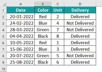
Step 1: The data provided consists of four columns: Date, Color, Unit, and Delivery.
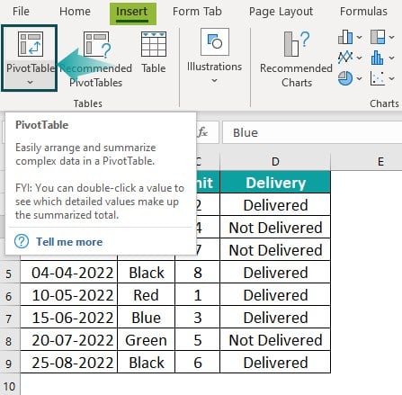
Step 2: To create a PivotTable, navigate to the Insert tab and select the PivotTable option, as demonstrated below.
Step 3: The Create a PivotTable window will appear upon clicking on the PivotTable option.
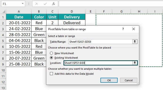
Step 4: In this window, we can select a table or a range to create the Pivot Table.

Step 5: We can place the PivotTable report in the same worksheet or a new one, as illustrated in the image above.
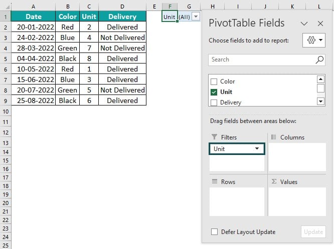
Step 6: The PivotTable Fields can be found on the right-hand side of the sheet, as shown below.
Step 7: We can observe the filter field within the PivotTable Fields. We can create a PivotTable filter by dragging the desired fields into the filters section. Let’s drag the Unit field into the Filters section. This action will generate a filter specifically for the unit.
Step 8: This filter allows us to easily sort and manipulate the Unit data according to our specific requirements. This method represents the standard approach for creating filters within a Pivot Table.
#2 – Create A Filter To Values Area Of An Excel Pivot Table
To create filters for those Pivot Table fields. It is worth noting that no filter option is available for value areas such as Count of Delivery and Count of Color. However, we can create filters, which can greatly assist us in making informed decisions.

To begin, we must select any cell adjacent to the table and click the Filter option in the Data tab.
Once we have activated the filter, it will appear in the Values area.
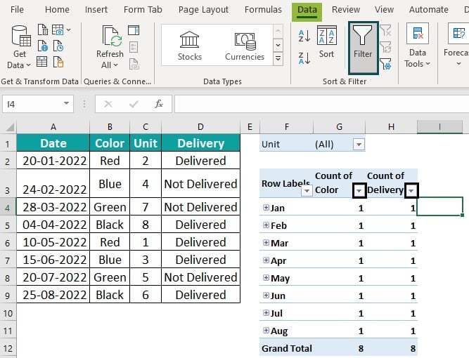
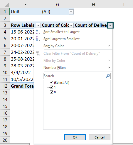
We can perform various operations on the value areas with the filters in place. We can sort them from largest to smallest to identify top sales figures, areas of focus, or any other relevant information. Similarly, we can sort from smallest to largest, sort by color, and even apply number filters such as <=, <, >=, >, and many more. These functionalities play a crucial role in the decision-making processes within any organization.
#3 – Display A List Of Multiple Items In A Pivot Table Filter
The previous example has provided us with insights on how to create a filter in a Pivot Table. Now, let us explore alternative methods of presenting a list distinctly.
There are three key approaches to displaying a list of multiple items in a PivotTable filter:
- Utilizing Slicers: Slicers offer an effective way to filter data in a Pivot Table visually. They provide a user-friendly interface allowing easy selection and deselection of specific items.
- Creating a list of cells with filter criteria: Another method involves generating a list containing the desired criteria. This approach lets users input their criteria directly into the cells, providing flexibility and customization options.
- Employing a list of comma-separated values: Lastly, a list of comma-separated values can be employed as a filter in a Pivot Table. This method involves listing the desired items separated by commas, allowing quick and straightforward filtering.
#4 – Using Slicers
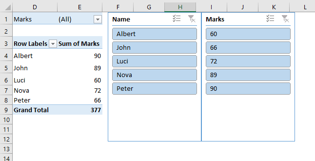
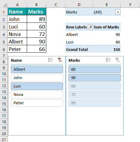
Let’s begin by creating a straightforward Pivot Table with two columns: Name and Marks.
Step 1: To create the PivotTable, follow these steps.
Select the data, go to the Insert tab, choose the PivotTable option, and create the PivotTable.

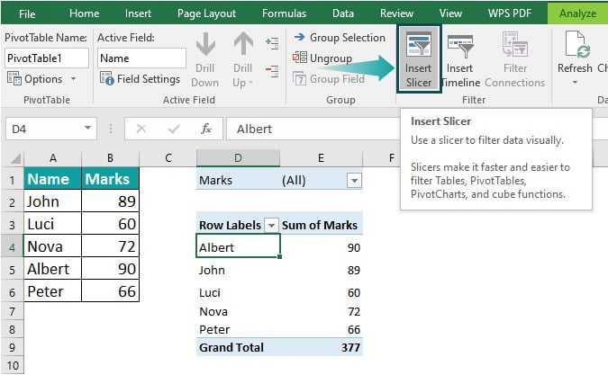
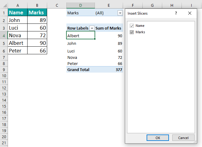
Step 2: Now, let’s explore the functionality of our filter using slicers in Pivot Table. By listing the filter criteria in slicers, we can easily see how they change based on our selection. To do this, select any cell within the Pivot Table, navigate to the Analyze tab on the ribbon, and click Insert Slicer.
Step 3: We need to insert the field we want to filter into the slicer. In this case, we’ll select the Function field and click OK. This action will add a slicer to the sheet.
The items highlighted in the slicer correspond to the filter criteria in the PivotTable’s filter drop-down menu.
Step 4: This simple solution effectively displays the filter criteria. We can easily filter out multiple items and observe how the results vary in the value areas. In the example below, we selected specific functions visible in the slicer. We determined the count of age categories for different industries (row labels dragged into the row label field) associated with those functions. We can see how the results adjust accordingly by changing the function as needed.
Step 5: If our list contains numerous items, it may become challenging to display them properly. We might have to scroll to see which items are selected. This leads us to the next solution: listing the filter criteria in cells.
Introducing the Create List of Cells With Pivot Table Filter Criteria feature, which comes to our rescue.
#5 – Create List Of Cells With Pivot Table Filter Criteria
We will utilize a connected PivotTable and the slicer above to establish a connection between two PivotTables.
Step 1: First, we create a duplicate copy of the existing PivotTable and paste it into an empty cell.
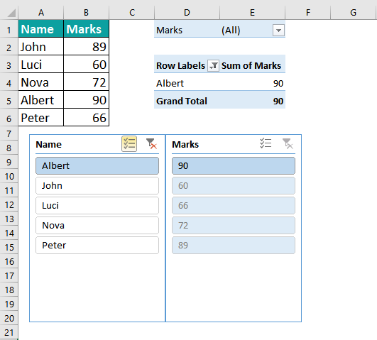
Step 2: We have a duplicate copy of our PivotTable, which we will modify slightly to display the Function field in the Rows area.
Step 3: To achieve this, select any cell within our PivotTable, navigate to the PivotTable field list, and remove the Industry from the Rows section. Additionally, we will remove the Count of Age category from the Values area and move the Function from the Filters section to the Rows area. This adjustment allows us to view a list of our filter criteria. Referring to the filter drop-down menu, we can observe the items in the slicers and function filters.
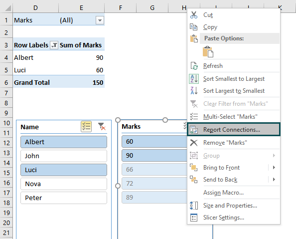
Step 4: By connecting both PivotTables through the slicer, we now have a comprehensive list of our PivotTable filter criteria. To confirm the connection, we can right-click anywhere on the slicer and access the PivotTable Connections menu.
Step 5: The PivotTable connections menu will display checkboxes indicating the connection between these PivotTables.
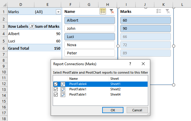
Step 6: This connection ensures that any changes made in the first PivotTable will automatically be reflected in the other.
Step 7: Furthermore, we can relocate PivotTables as needed. For instance, we can incorporate them into financial models and modify row labels accordingly.
#6 – List Of Comma Separated Values In Excel Pivot Table Filter
One way to display our PivotTable filter criteria is by using a single cell with a list of comma-separated values. This can be achieved using the TEXTJOIN function introduced in Excel 2016. If we use a version before 2016, we can also use the CONCATENATE function.
The TEXTJOIN function offers three different arguments that we can utilize.
Step 1: Firstly, the delimiter argument allows us to specify the character that will separate the values, such as a comma or space.
Step 2: Secondly, the ignore empty argument can be set to TRUE or FALSE, depending on whether we want to exclude blank cells.
Step 3: Lastly, the text argument allows us to add or specify a range of cells containing the values we wish to concatenate.
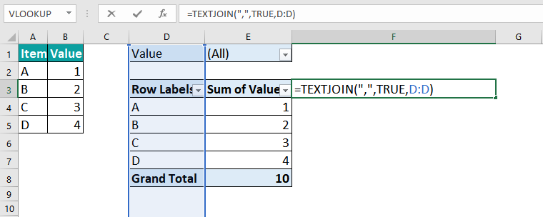
Step 4: To implement the TEXTJOIN function, we can type the formula with the desired delimiter (in this case, a comma), set the ignore empty argument to TRUE, and specify the range of cells that contain the selected items from the filter.

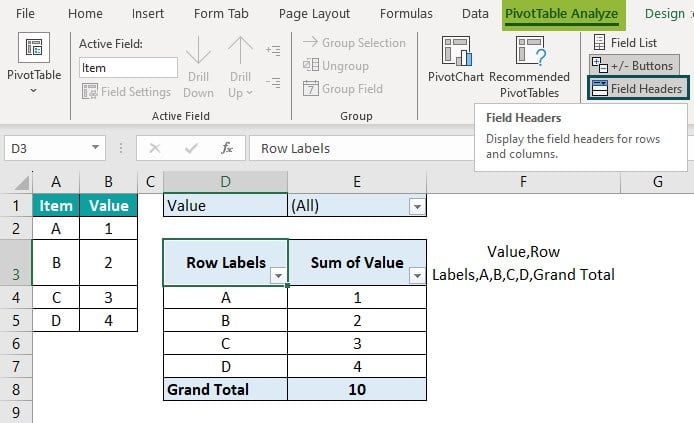
Step 5: By doing so, we obtain a comma-separated list of all our PivotTable filter criteria. We can hide the cell if we prefer not to display these filter criteria in the formula. This can be done by selecting the cell, navigating to the Analyze options tab, and clicking Field Headers.
Important Things To Note
- The pivot table filter is a powerful tool for professionals to manipulate and analyze large data sets efficiently.
- Users can easily sort and summarize information according to specific criteria, enabling them to gain valuable insights and make informed decisions.
- Its versatility lies in enabling multiple filtering options, such as choosing particular values or ranges, applying labels or colors to highlight key data points, or creating custom filters with advanced conditions.
- The professionals can tailor the pivot table view to their needs and focus on analyzing the relevant data subsets effortlessly.
- The pivot table filter is particularly beneficial when dealing with complex datasets where granular analysis is required across various dimensions and variables simultaneously.

Frequently Asked Questions (FAQs)
A pivot table filter is an invaluable tool in data analysis due to its capability to isolate and examine specific subsets of data. In complex datasets of numerous variables and dimensions, filtering lets analysts focus on the most relevant information, eliminating noise and enhancing clarity. A pivot table filter allows users to zoom in on a specific segment for closer scrutiny by selecting particular criteria, such as periods, product categories, or geographical regions. This facilitates the identification of patterns, trends, or anomalies that would otherwise remain hidden amidst vast amounts of data.
Professionals can employ several advanced tips and tricks to streamline their data analysis process when using pivot table filters more effectively.
• First, utilize the Top 10 filter option; this feature is particularly valuable when identifying top-selling products or underperforming segments.
• Secondly, the “Value Filters” feature enables users to specify criteria such as greater than, less than, or between certain values.
• Moreover, incorporating time-based filtering options in pivot tables can enhance insights by comparing trends over different periods or analyzing data within particular time frames.
• Lastly, employing advanced filtering techniques such as using multiple filters simultaneously in pivot tables.
When using pivot table filters, there are indeed certain limitations and restrictions that should be considered.
• Firstly, it is important to note that pivot table filters can only be applied to the data within the specific variables or fields included in the pivot table.
• Furthermore, some data types, such as text or string values, may not be suitable for filtering as they lack the numerical characteristics required for comparisons.
• Moreover, it is crucial to consider potential cascading effects when applying multiple filters simultaneously, which could inadvertently exclude certain relevant data from the analysis.
• Finally, advanced filtering options like color or icon-based criteria are not available within pivot tables and might require an alternative approach for implementation.
Download Template
This article must help understand Pivot Table Filter formulas and examples. We can download the template here to use it instantly.
Recommended Articles
Guide to Pivot Table Filter. Here we learn how to filter in a pivot table with steps, examples & downloadable excel template. You can learn more from the following articles –

Leave a Reply