
What Is A Pivot Table Slicer?
The pivot table slicer is a filter type used with pivot tables containing a massive amount of data. And the option makes analyzing and understanding the data extracted and shown in a pivot table more straightforward.
Users can add a slicer to a pivot table to check the fields which are visible and hidden in the pivot table. And hence, the option helps maintain data integrity and security.
Use this Pivot Table Slicer Template to follow along with the examples in this article.
Download Excel TemplateFor example, the image below shows a dataset containing the sales representatives and details about the products they sold and the sales they generated.
Also, the image shows the pivot table created for the given dataset using the PivotTable option in the Insert tab.

If adding slicer to pivot table,shown above, based on the Sales Representative, is the requirement.
Then, we can use the Insert Slicer option in the Analyze tab. It will enable us to select the category for the slicer, Sales Representative.

And clicking OK will add the required Sales Representative slicer to the worksheet.
Also, the above is a pivot table slicer multiple columns example, as we created a slicer with more than one column using the Columns settings in the Options tab.
After adding slicer to pivot table, we can click the sales representatives’ names in the slicer to filter and display their sales information in the pivot table.
Key Takeaways
- A pivot table slicer is a filtering option containing buttons to filter and display the required data in pivot tables quickly. Also, the option shows the existing filter conditions applied to pivot tables, which helps understand the displayed and hidden data in the pivot table.
- Users can connect a slicer to one or more pivot tables to use them as movable filters.
- We can insert a slicer for a pivot table using the Slicer option in the Insert tab, the Insert Slicer option in the Analyze tab, and from the PivotTable Fields window.
How To Create A Pivot Table Slicer In Excel?
We can create a pivot table slicer in Excel using the following methods:
- From the Insert Tab
- From the Analyze Tab
- From the PivotTable Fields Pane
But before we see the abovementioned methods to add a pivot table slicer, we shall see the steps to create a pivot table.
- First, we must create a pivot table for the entire dataset. Next, click on a cell within the dataset range. Otherwise, select the required dataset range. And then, select the Insert tab → Choose the PivotTable option to open the Create PivotTable window.


[Alternatively, we can select the required data and apply the keyboard shortcut Alt + N + V to open the Create PivotTable window]
- Next, as we select the source data and open the Create PivotTable, the first field, Table/Range, will get updated automatically. And we can choose where to display the pivot table using the Location field.
- Finally, click OK to view the required pivot table.
Now, we shall see the methods to create a pivot table slicer in Excel.
Method #1 – From The Insert Tab
First, click in the pivot table → Select the Insert tab → Choose the Slicer option to open the Insert Slicers window.

Method #2 – From The Analyze Tab
To begin with, click on the pivot table.
Next, select the Analyze tab. Then, choose the Insert Slicer option to open the Insert Slicers window.

The above mentioned methods will open the Insert Slicers window.

Next, select the field based on which we require the slicer for the pivot table.

Finally, clicking OK will display the required slicer for the pivot table.

Method #3 – From The Pivot Table Fields Pane
First, click the pivot table to make the PivotTable Fields window visible. And then, right-click the field based on which we must create the slicer from the fields listed in the PivotTable Fields window → Choose the Add as Slicer option from the menu.

Basic Example
Let us see an illustration for creating a slicer for a pivot table.
The table below lists students and their Mathematics and Science scores.

If the requirement is to build a pivot table for the given data and add a slicer for the pivot table based on the Subject field. Then, the steps are as follows:
- First, to build the pivot table for the entire dataset, click on a cell within the dataset range. Otherwise, select the required dataset.
And then, select Insert → PivotTable to open the Create PivotTable window.

- Next, check and ensure the input data range in the first field is correct, and choose the location to display the pivot table.
In our case, we shall display the pivot table in the current worksheet in cell A23.

Then, click OK to open the PivotTable Fields pane, and we will see the space in cell A23 to build the required pivot table.
- Next, click on the required fields listed in the PivotTable Fields window, one at a time, and drag them to place them in the required sections to obtain the below pivot table.
- Then, select cell A24 and update the column heading as Student.

Now, select cell B23 to update the filter name as Subject.
The above step will make the pivot table clearer. - Next, click on a cell within the pivot table. Then, select Insert → Slicer to open the Insert Slicers window.

[Alternatively, click on a cell within the pivot table and choose Analyze → Insert Slicer.
The Insert Slicers window will open]
- Now, select Subject from the fields in the Insert Slicers window and then, click OK.

[Alternatively, click the pivot table to make the PivotTable Fields window visible and right-click on the Subject field listed in the window. And select the Add as Slicer option from the pop-up menu.
This method will directly add the Subject-based slicer to the pivot table.]
Now, we can click the subject name in the slicer, for which we need to check the students’ scores in the pivot table.
For instance, clicking the Science option in the slicer will filter and display the chosen subject data in the pivot table, as shown below.


Examples
Check out the following pivot table slicer examples to understand its practical uses.
Example #1 – Display State-wise Population For The USA
We shall see a pivot table slicer multiple columns example.
The table below shows the US state-wise population statistics.

The requirement is to build a pivot table for the given data and add a slicer with multiple columns. Then, the steps are as follows:
- Step 1: First, we must create the pivot table for the entire dataset. So, we can click on a cell within the dataset range. Otherwise, we must select the required data range for inserting the pivot table.
And then, select Insert → PivotTable to open the Create PivotTable window.
- Step 2: Next, ensure the source data range updated in the first field in the Create PivotTable window is correct. And enter the location where we must display the pivot table.

Clicking OK will show the PivotTable Fields window and the space to insert the pivot table.

- Step 3: Then, drag the required fields listed in the PivotTable Fields window in the respective sections in the pane.

- Step 4: Now, select cell range C14:C23 and click Home → Number Format → More Number Formats to open the Format Cells window.

Next, select the Number category in the Number tab and set the number format of the population figures the same as the source data.

And click OK.

Next, select cell A13 and update the column name to US State.

And then, click the first field in the Values area in the PivotTable Fields window and select the Value Field Settings option to open the Value Field Settings window.

Now, update the Custom Name field to show a customized name for the selected field in the pivot table. And click OK.

And iterate the previous action for the second field in the Values section in the Pivot Table Fields window.


Step 4 will make the pivot table more understandable.
- Step 5: Next, click the pivot table to enable the Analyze tab and then, select the Insert Slicer option to open the Insert Slicers window.

Now, select the US State field and click OK in the Insert Slicers window.

- Step 6: Next, the US State-based slicer will appear as below. And as it is selected, the Options tab appears in the ribbon.

Next, set the Columns field as 2 in the Options tab to show two columns in the slicer and achieve a slicer with multiple columns.

Next, with the slicer selected, drag the slicer border to expand it and show the state names clearly.


Now, we can click the state name in the slicer for which we wish to filter and show the data in the pivot table.

Furthermore, we can click the Multi-Select icon or press the shortcut keys Alt + S to select multiple options.
Then, the chosen states’ data will get filtered and displayed in the pivot table.

Finally, we can click the Clear Filter icon to clear the applied filter in the slicer.

Example #2 – Weekly Price Change For Top 5 Cryptocurrencies
Let us see how to create a pivot table slicer search box with an example.
The table below shows the weekly price change for the top five cryptocurrency companies in percentage.

Now, to create a pivot table slicer search box, the steps are:
- Step 1: To start with, click on a cell within the given dataset. Then, select Insert → PivotTable to open the Create PivotTable window.

- Step 2: Next, ensure the source data range updated in the first field in the Create PivotTable window is correct. And enter the location where we must display the pivot table.

Clicking OK will show the PivotTable Fields window and the space to insert the pivot table.

- Step 3: Now, drag the fields listed in the PivotTable Fields window in the respective sections in the pane.

- Step 4: Then, select cell range B24:B28. Next, choose Home > Number Format > Percentage to show the weekly price change figures in percentage.

Next, select cell A23 and update the column heading as Week.

Step 4 will ensure the pivot table is more meaningful.
- Step 5: Now, click the pivot table to enable the Analyze tab. Then, select Insert Slicer to open the Insert Slicers window.

Next, check the Cryptocurrency Company field box and click OK in the Insert Slicers window.

We will obtain the Cryptocurrency Company-based slicer.

And then, with the slicer selected, drag its border outward to expand it so that the slicer title is visible.

- Step 6: Then, move the slicer to create space for copying and pasting the pivot table again to form the search box for the slicer.

Moving the slicer shows a pivot table slicer vs filter comparison factor. While we can move slicers according to our requirements, we cannot move a filter. Because, it remains locked with a column and row.
Next, select the entire pivot table and press Ctrl + C to copy it. And select cell E23 and press Ctrl + V to paste the pivot table.

- Step 7: Next, click the pivot table in cell E23 to enable the PivotTable Fields window. Then, unselect the fields in the PivotTable Fields window to clear them from the respective sections.

Next, drag the Cryptocurrency Company field to the Filters section in the PivotTable Fields window.
We perform this action because the added slicer is Cryptocurrency Company field-based, and we require the search box for the same field.

And then, select the pivot table filter in cell range E21:F21 and press Ctrl + X to cut it.

Now, select cell E23 and press Ctrl + V to paste the filter in the target cell range E23:F23.

- Step 8: Next, select cell F23 and right-click to select PivotTable Options from the context menu.

The PivotTable Options window opens, where we must unselect the option highlighted in the image below to avoid column width autofit on update and click OK.

This step will ensure that the chosen cell’s column width will remain the same when we select an option using the drop-down button. However, the cell column width will be adjustable.
- Step 9: Now, drag the slicer to column F and adjust the column F width so that the slicer and the field’s drop-down button display, as shown below.

Next, click the column E header and right-click to select Hide from the context menu to hide the column.


Now, when we click the drop-down button, the search box appears, giving the appearance of a slicer search box for the pivot table.
Next, we can click on a company name and OK in the search window to filter and display its weekly price changes in weeks 1-4 in the pivot table.

The above step will show the selected company name in the slicer and its data in the pivot table.

Furthermore, clicking the key E on the keyboard will show the cursor in the search box, where we can type the company name. And then click OK to apply the filter.


Thus, comparing pivot table slicer vs filter shows that we can connect a slicer to multiple tables.
Now, we can click the slicer to enable the Options tab and use the Report Connections option to confirm to which all pivot tables the slicer is currently connected.


On the other hand, a filter can connect to only one pivot table.
Example #3 – Multiple Slicers
We shall see how to create multiple slicers for a pivot table.
The table below lists items, their categories, the order delivery destinations, and units ordered data.

Now, the requirement is to create multiple slicers for the pivot table based on the given data. Then, the steps are as follows:
- Step 1: To start with, click on a cell within the dataset range and then, select Insert à PivotTable.

- Step 2: Next, the Create PivotTable window opens. Here, we must confirm the updated source dataset range in the first field is correct. And then, we must enter the location where we wish to display the pivot table.

Now, click OK to open the PivotTable Fields pane and then, create the space to insert the pivot table.

- Step 3: Then, drag the fields listed in the PivotTable Fields window in the required sections, as shown below.

- Step 4: Next, select cell A19 and then, update the column heading as Order Delivery Destination.

Now, select cell B18 and update the Column Labels cell as Item to make the pivot table understandable.

- Step 5: Next, click the pivot table to enable the Analyze tab and then, select Insert Slicer to access the Insert Slicers window.

- Step 6: Now, select the Item field and click OK in the Insert Slicers window to create an Item-based slicer.


Next, repeat step 6 to add the Category and Order Delivery Destination-based slicers.


Thus, the multiple slicers added for the pivot table will appear as shown below.

Now, we can now choose the options in the respective slicers to extract and display the required information in the pivot table based on the applied filters in the slicers.

Important Things To Note
- To correctly use the added pivot table slicer, carefully drag the column fields and place them in the correct sections or areas in the PivotTable Fields window.
- When creating a slicer for multiple pivot tables, ensure the slicer is connected to the pivot tables. And we can click the slicer to enable the Options tab and use the Report Connections option to confirm the connections.
- Click the Multi-Select icon to select multiple options in a slicer. And click the Clear Filter icon in the slicer to clear the applied filter.
Frequently Asked Questions (FAQs)
• Slicers can connect multiple pivot tables.
• We can filter pivot tables quickly using slicers’ buttons.
We can create a pivot table date range slicer. The table below shows a list of employees and their tasks’ completion status.
The steps to create pivot table date range slicer are:
• Step 1: To begin with, click on a cell within the dataset range and select Insert → PivotTable.
• Step 2: Next, the Create PivotTable window opens, where we must confirm the source data range entered in the first field is accurate. And then, we must update the location where we wish to display the pivot table.
Click OK. The PivotTable Fields pane opens and show the space to insert the pivot table.
• Step 3: Now, let us drag the required fields listed in the PivotTable Fields window to the respective sections so the pivot table shows the employees’ task status.
• Step 4: Then, select cell A16 and update the column name as Name.
Next, select cell B15 and update the Column Labels cell as Task Status to make the pivot table easier to understand.
• Step 5: Next, right-click the Task Completion Date in the PivotTable Fields window and choose the option to add the chosen field as a slicer from the menu.
The above step will result in the date-based slicer.
Next, click the slicer and drag its border to make its title visible clearly.
Now, we can click on the required dates in the slicer to filter and then, display the task submission details on the chosen dates in the pivot table.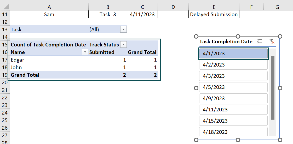
Thus, in this way, we can select a date field from the given list of fields in the PivotTable Fields window and add it as a slicer for the pivot table.
Slicers can be used without a pivot table. However, we must have an Excel table to use the Slicer option from the Insert tab to insert slicers in Excel.
Use this Pivot Table Slicer Template to follow along with the examples in this article.
Download Excel Template