
What Is GetPivotData In Excel?
GetPivotData in Excel is a function that helps us get the record from the pivot table based on the various criteria given in the formula. GetPivotData in Excel is one of the lookup functions specifically designed to work with pivot table summary data.
In simple terms, GetPivotData in Excel is used as a query statement for fetching the data from the pivot table based on the table structure instead of the excel cell reference.
Use this GetPivotData In Excel Template to follow along with the examples in this article.
Download Excel TemplateFor example, look at the following pivot table summary in Excel.
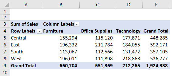
We have Region-wise (in rows) and Category-wise (in columns) sales summary reports. Assume we need to get the value for the region ‘East’ and the category ‘Technology’ outside the pivot table.
Type the equal sign outside the pivot table and select cell D6.
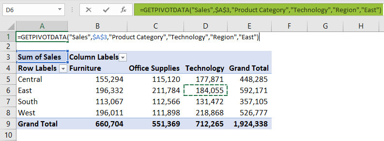
As we can see, as soon as we select a cell from the pivot table, it automatically inserts the GetPivotData in Excel function with auto-filled arguments. We will look into the arguments of the GetPivotData in Excel function in detail in the later part of the article.
Hit the Enter key, and we will get the sales value for the region ‘East’ and the category ‘Technology.’
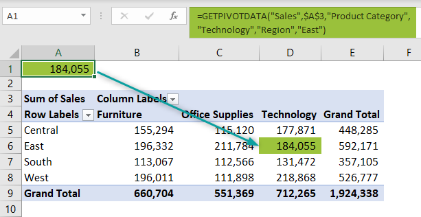
In the formula bar, we can see the GetPivotData in Excel function.
Key Takeaways
- The GetPivotData can retrieve the value from the pivot table based on the columns and items.
- The function automatically takes the fields and items if we just select the cell from the pivot table by entering an equal sign in the empty cell.
- The GetPivotData takes cell references for item names, and when the cell reference is given, we need not have to enter those in double-quotes.
- If we type an equal sign in an empty cell and select any of the cells from the pivot table, the GetPivotData function will be applied automatically.
- We can turn off and turn on the GetPivotData formula.
GetPivotData() Excel Formula
The syntax of GetPivotData formula is

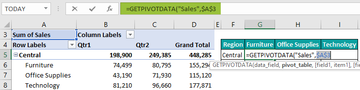
Let us understand the syntax of the GetPivotData Excel formula with the following example. We have the following pivot table in an Excel spreadsheet.

In cell G7, we have applied the GetPivotData function.
Data Field: The first argument is mandatory. The Data field is nothing but the aggregate value we are looking for. For example, in the above pivot table image, we are looking for the sales value aggregation. Hence, ‘sales’ becomes the data field.
Pivot Table: For this argument, we can choose any cell of the pivot table area to insist on the formula to search in this pivot table. In the above example, we have given cell A3 as a reference.
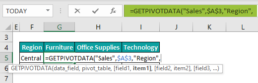
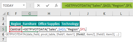
Field 1: This is from the field (row) of the pivot table we are looking for the value. In the above example, we have given the filed 1 name as ‘Customer Segment.’ In simple terms, ‘Customer Segment’ is the column we have in the data table.
Item 1: This is from the selected field 1, the value we are looking for. In the above example, we have given the item as ‘Home Office,’ i.e., from the ‘Customer Segment’ column, we are looking only for the ‘Home Office’ value.
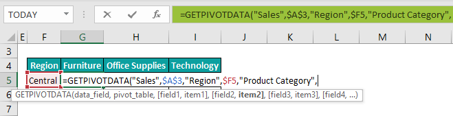
Field 2: This is from which field (column) of the pivot table we are looking for the value. In the above example, we have given the filed 2 names as ‘Product Category,’ i.e., ‘Product Category’ is the column in the data table.
Item 2: This is from the selected field 2, which value we are looking for. In the above example, we have given the item as ‘Technology,’ i.e., from the ‘Product Category’ column, we are looking only for the ‘Technology’ value.
Note: We can provide 126 fields and items.
How To Use GetPivotData In Excel – Basic Example
First, we will look at a basic example of applying GetPivotData formula.
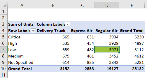
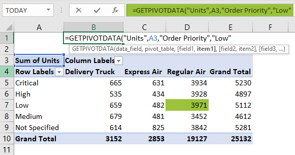
Consider the following pivot table.
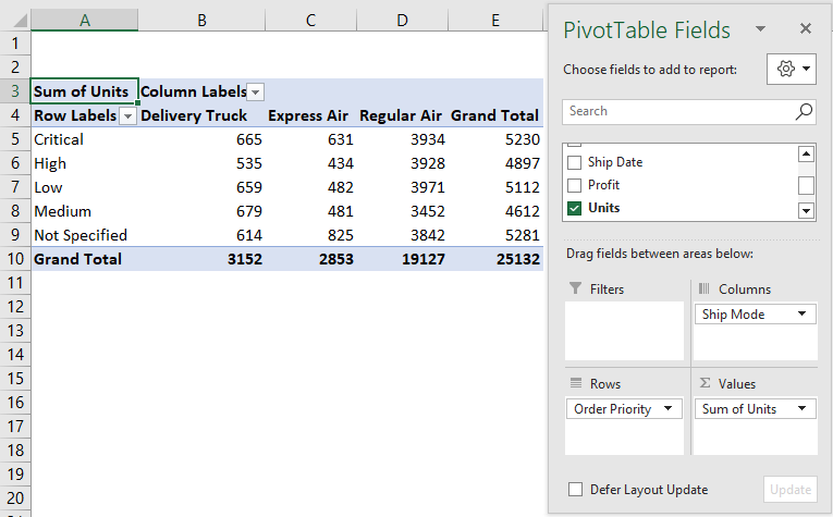
The above pivot table shows the units sold based on order priority and ship mode.
Assume we need to know the value for the order priority ‘Low’ and ship mode ‘Regular Air.’
We will use GetPivotData in excel to retrieve this information from the above pivot table. Please do follow the steps listed below:
Step 1: Enter the GetPivotData function in any of the empty cells.
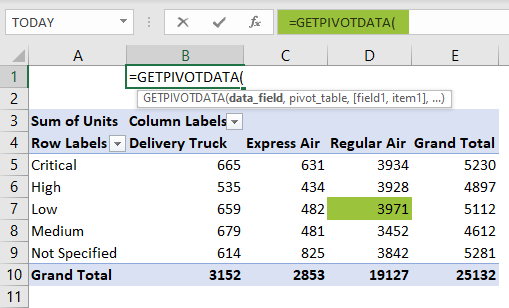
Step 2: The first argument is the data field, i.e., what aggregated information we need from the above pivot table. So, this will be the number of units sold. Enter this criterion in double-quotes.
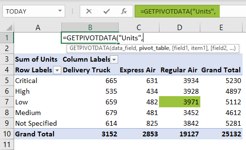
Step 3: Next argument is Pivot Table, i.e., from which pivot table we need to retrieve the value. Hence select any of the cells from the pivot table area.

Step 4: Next, we need to provide the field name. The first field name we are looking for is ‘Order Priority.’ Enter this field name in double quotes.
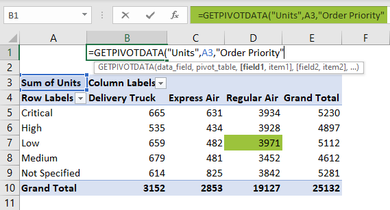
Step 5: Next, we need to provide the item from the selected field, i.e., from the entered field, which item we are looking for. So, this will be ‘Low.’
Step 6: Next, we need to provide the second filed name, i.e., ‘Ship Mode.’
Enter ship mode in the field 2 argument.
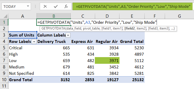
Step 7: For item 2, we need to give the item from field 2 as ‘Regular Air.’

Step 8: Now, all the fields and items are provided. Close the bracket and hit the Enter key to get the result in cell B1.
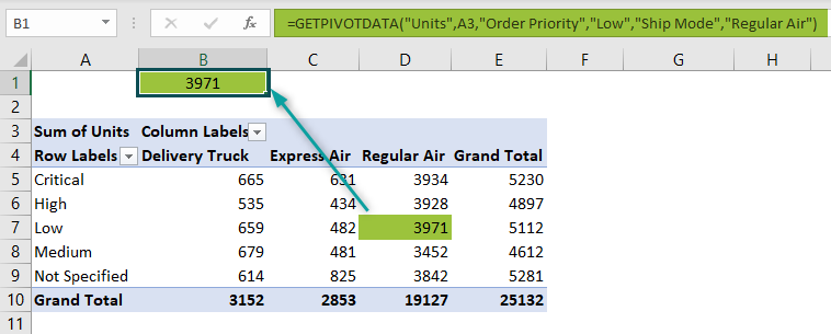
The result in cell B1 is 3971, It indicates the number of units sold for order priority ‘low’ and ship mode ‘regular air.’
This way, we can use GetPivotData in Excel and retrieve the specific value from the pivot table fields.
Examples
Example – 1 – Apply GetPivotData For Date Columns
Continuing with the same data from the above example, we have inserted another pivot table for the same data.

In the above pivot table, we have date-wise sales. We will insert GetPivotData in Excel function to retrieve the value for the specific date.
Assume we need to get the sales for the date 01-Feb.
Enter an equal sign in any empty cells and choose the cell for 01-Feb.
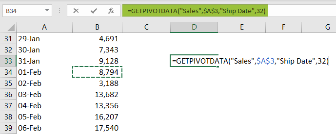
When we choose the cell from the pivot table, it automatically applies the GetPivotData formula with all the necessary auto-filled arguments.
However, we can see that the date is selected.
It has selected the date as 32, where we have selected the cell of date 01-Feb. Since January has 31 days, by default, February 1st will be treated as the 32nd day. Therefore, it has taken the item name as 32, not as ‘01-Feb.’
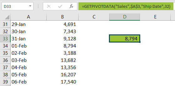
By looking at item 32, a new user cannot identify which date data it is showing up. Hence, it is better to provide the date field.
Enter the date excel function and provide the date as shown in the following image.

The result for 01-Feb is 8794, which is returned from GetPivotData in Excel function. So, now any user can understand that the GetPivotData function is returning the value for the day 01-Feb.
Example – 2 – Create A Modified Summary Table Using GetPivotData
Continuing with the same data from example #1, we have inserted a pivot table, as shown in the following image.

Assume, from the above table, we need to fetch a few values, and we have designed the table like the following.
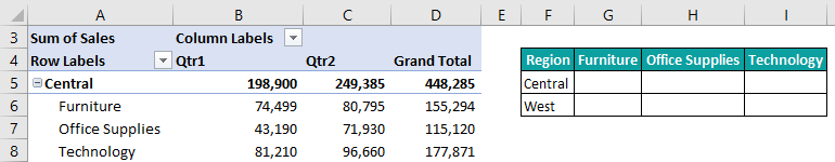
So, we need to know the total sales for regions Central and West for each product category.
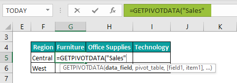
Step 1: Enter the GetPivotData in Excel function in cell G5.
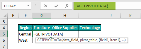
Step 2: The data field we need from the pivot table is ‘Sales,’ so enter this field name in double quotes.
Step 3: Choose any cells from the pivot table field and make it an absolute reference by pressing the F4 key once.
Step 4: Enter the filed 1 name as ‘Region.’
Step 5: For the item 1 argument, choose the cell F3 and make the column reference absolute by pressing the F4 key thrice.
Step 6: Next, enter the field 2 name as ‘Product Category.’
Step 7: For the product category item, choose the cell G2 and make the row reference absolute by pressing the F4 key twice.
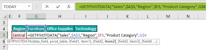
Now, all the required fields and items are entered into the formula. Finally, close the bracket and hit the Enter key to get the result.
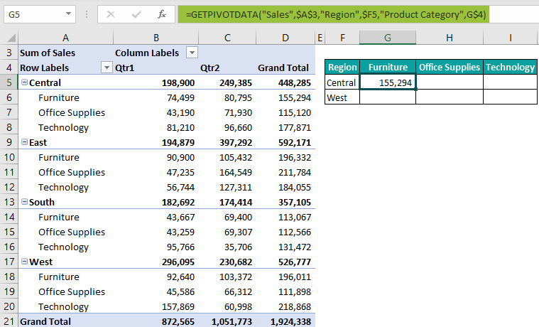
Step 8: Copy and paste the formula to all the remaining cells to get the value for all the cells.
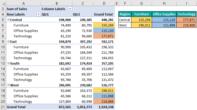
We have the respective values for each region and category (colored in the same colors in the pivot table for better understanding).
Important Things To Note
- The GetPivotData in Excel returns the #REF (reference error) if any of the field name or item name doesn’t match with the records of the pivot table.
- In the GetPivotData function, columns are referred to as fields, and rows are referred to as items.
- We can provide up to 126 fields and items for the GetPivotData functions.
- The function GetPivotData works only for pivot table data.
- When we enter them directly in the formula, all the pivot table fields and items should be supplied in double-quotes.
- The GetPivotData function returns results only from the available fields in the pivot table.
Frequently Asked Questions (FAQs)
We can add two GetPivotData in Excel. For instance, we have the following pivot table in Excel.
To get the sales value of region ‘East’ and product category ‘Office Supplies’, we can apply the following GetPivotData function.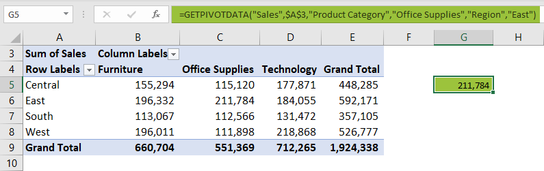
Assume we need to get the sales of the regions ‘East’ & ‘West’ and for the product category ‘Technology’ we can apply GetPivotData functions in one.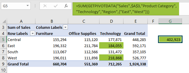
In the item argument of the region field, we have applied two regions East and West, in curly brackets and then surround the GetPivotData function in the SUM function.
We can also apply two GetPivotData functions and add them together to the result.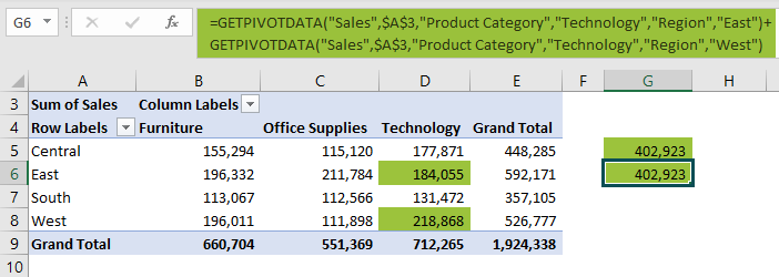
After the first GetPivotData function, we added plus symbol and then applied another GetPivotData function to get the same result as the previous one.
By default, when we select any of the cells in the pivot table, the GetPivotData function will be automatically applied as shown in the following image.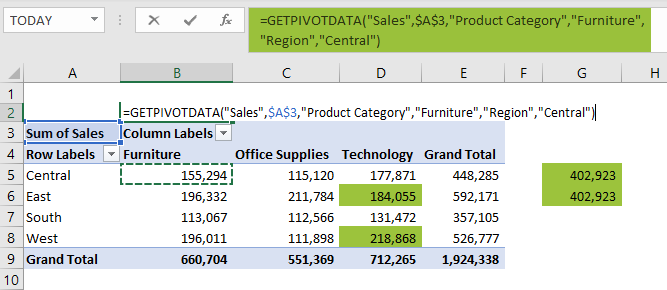
However, we can disable this with just a click.
Select any of the cells in the pivot table, and it will activate Pivot Table Analyze tab. Under this tab, click on the Pivot Table drop-down and also click on the Options drop-down.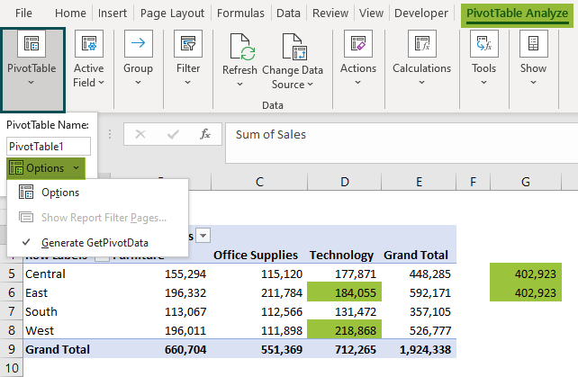
As we can see in the above image, Generate GetPivotData is enabled. Click on this option, and the tick mark disappears, as shown in the following image.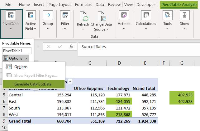
Now, if we select any of the cells in the pivot table, Excel no longer applies the GetPivotData function automatically.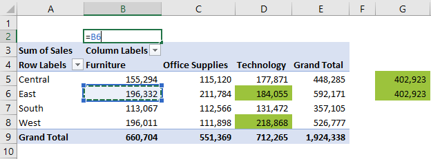
Type an equal sign in any of the cells in the new sheet and go to the pivot table sheet and choose any of the cells in the pivot table. The moment we choose a cell in the pivot table, it will automatically insert GetPivotData in excel.
From the detailed summarized report, sometimes we may have to look at only one specific record, so in these cases we use GetPivotData in excel.
Use this GetPivotData In Excel Template to follow along with the examples in this article.
Download Excel TemplateRecommended Articles
Continue with these related resources when you want the next practical step in this topic.
Explore the full Excel Tables and Data Tools guide or browse Excel Resources.