
What is ISBETWEEN in Google Sheets?
The ISBETWEEN function checks whether a given number lies between two specified values, which also include the endpoints. It returns TRUE if the number falls within the given range and FALSE otherwise. We use ISBETWEEN in Google Sheets to find if a value falls within thresholds, evaluate ranges, or validate inputs, where we can check if a value is within a range, such as passing an exam. It helps simplify complex nested IF or comparison statements and is valuable in both data validation and conditional formatting.
As an example, let us check if a student’s test score of 67 is between 60 and 90 (inclusive). We use the following formula for it:
=ISBETWEEN(67, 60, 90)

This formula returns TRUE, thereby indicating that the score falls within the specified range. If the number were outside the range (e.g., 58), the formula would return FALSE.
Use this ISBETWEEN in Google Sheets Template to follow along with the examples in this article.
Download Excel TemplateKey Takeaways
- The ISBETWEEN function checks whether a value lies between two specified numeric bounds, including the endpoints. It returns TRUE if the condition is met and FALSE otherwise.
- The syntax of the function is as follows:
- =ISBETWEEN(value, lower_bound, upper_bound, [lower_value_is_inclusive], [upper_value_is_inclusive])
- It is commonly used in grading, inventory checks, threshold validations, and date or time range analysis to simplify logical conditions.
- ISBETWEEN only works with numeric values or values like dates, which are stored as serial numbers.
- The lower bound must come before the upper bound; reversing them will result in a #NUM! error.
Syntax
Now that we have a basic idea of how the function can be used, let us look into the ISBETWEEN formula in Google Sheets to understand how to use ot for specific scenarios. The syntax of ISBETWEEN in Google Sheets is as follows:
=ISBETWEEN(value_to_compare, lower_bound, upper_bound, [lower_value_is_inclusive], [upper_value_is_inclusive])
- value_to_compare – The number we will test.
- lower_bound – The minimum value of the range (inclusive).
- upper_bound – The maximum value of the range (inclusive).
- [lower_value_is_inclusive]: (Optional) A Boolean value. If TRUE, the lower bound is included in the range. If FALSE, it’s excluded.
- [upper_value_is_inclusive]: (Optional) A Boolean value. If TRUE, the upper bound is included in the range; else it is not included.
The function returns TRUE if the value argument is greater than or equal to the lower_bound argument and less than or equal to the upper_bound. Otherwise, it returns FALSE. The inclusivity of the upper and lower bounds depends on the optional arguments, but by default, both upper and lower bounds are included.
How To Use ISBETWEEN Function in Google Sheets?
As seen before, the ISBETWEEN function is used to determine if a value falls within a specified range, which also includes the endpoints. We may have to use it in several scenarios where we have to check if a value falls within a range, to evaluate results accordingly. In such scenarios, there are two common ways to use this function.
- By typing ISBETWEEN directly into the cell
- Selecting ISBETWEEN through the menu options
Let’s go through the manual method first step by step using a real-time example.
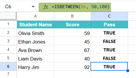
Given below is a list of students’ scores, and we must find if they fall within the passing range. Here, the students must score above 50% for a pass.
Step 1: Prepare the data by entering all the details in a Google Sheets as shown below.

Step 2: Enter the ISBETWEEN Formula. For this, go to Column C2 where you want to see the result. Type the formula as follows:
=ISBETWEEN(B2, 50,100)

This checks if the score in cell B2 is between the values 50 and 100.
Step 3: Press Enter. Check the result. The formula will return TRUE if the score is between 50 and 100 and FALSE otherwise.

Step 4: Drag the fill handle down to apply the formula to the rest of the rows.
Using the Menu Bar
If you find using the menu easier, go through the following steps.
- Select the target cell, which is C2 in this case.
- Go to Insert > Function > Logical > ISBETWEEN
- Google Sheets will insert =ISBETWEEN(). Fill in the arguments manually and press Enter to see the result.
Examples
To better understand how the ISBETWEEN function works in practical scenarios, let’s explore a few examples using some real-time data. These examples demonstrate how to check if a value falls within a specific range. Such examples could include determining if a score qualifies as a pass, if a temperature is within a safe limit, or if a date falls within a specified interval.
Example #1
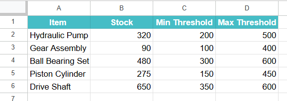
In this example, let us evaluate if some products’ stock levels are within a safe threshold. It is very important in warehouse management to check if items are in the right stock. We must check if they are either too low or too high in stock. A safe stock range is set between the values specified in Columns C and D for each item. Let us use ISBETWEEN in Google Sheets to check if the products’ stock level is within this range.
Here, we are not just checking the stock but implementing an inventory control logic that helps warehouse managers focus on stock items that are either overstocked or understocked.
Step 1: Enter the following details in a sheet, as shown below.
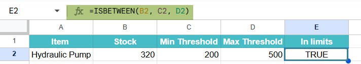
Step 2: Enter the ISBETWEEN formula to check if the current stock is within the required range. Enter the following formula in Google Sheets.
=ISBETWEEN(B2, C2, D2).

Here, we have the lower and upper bounds of each product in columns C and D, respectively. We also have the stock count in Column B.
This formula will return TRUE if the stock level is between 100 and 500 units (inclusive).
Step 3: Press Enter. Once you press Enter, the cell shows TRUE, as the value of the product is 320 units which is within the safe range.
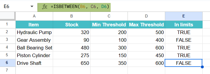
Drag the formula for all the other items.
The results will filter out stock items that are either too low or too high. Using ISBETWEEN, such logic becomes scalable across hundreds of products.
Example #2 – Using ISBETWEEN with IF Formula
In a village, the village head tries to separate the population as adults or Child based on the people’s ages. He has an entire list of people. Let us look at how this can be done using ISBETWEEN with IF.
Step 1: Enter all the details in a sheet, as shown below.
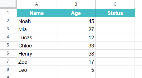
Step 2: Let us use the following function to classify each person as a child or an adult.
Here, the ISBETWEEN checks if the person’s age in Column B is between 0 and 17. If so, the IF function prints “Child”, else prints “Adult.”
=IF(ISBETWEEN(B2, 0, 17), “Child”, “Adult”)

Step 3: Press Enter. Drag the formula for the other values as well.

Example #3 – Using ISBETWEEN with FILTER Formula
We have an interesting example where we have some employees who are eligible for a bonus if their joining dates are within a specified range, If so, it returns TRUE, and FALSE otherwise. We often use ISBETWEEN with the FILTER function to conditionally display data based on whether values are within a certain range.
The syntax of the FILTER function in Google Sheets is as follows:
=FILTER(range, condition1, [condition2, …])
range: The Google Sheets ISBETWEEN data range you want to filter.
condition1, condition2, …: Boolean expressions that specify which rows to include in the filtered output.
Let us use it in combination with ISBETWEEN.
Step 1: Set up your data: Enter the names in Column A and the joining dates in Column B.

Step 2: Use the formula shown below.
=FILTER(A2:A8, ISBETWEEN(B2:B8, F1, F2))

This formula filters column A values based on the condition that the corresponding dates in column B are between the start and end dates specified in cells F1 and F2.
Step 3: Press Enter.

The FILTER function will return a new range containing only the values from column A where the dates in column B fall within the specified range.
Important Things to Note
- ISBETWEEN returns TRUE if the value is equal to the lower or upper bound, as the end values of the range are also included by default.
- ISBETWEEN works only with numeric values. If you use it with text and other values, it can cause errors or unexpected results.
- If any of the inputs are blank cells, the function may return incorrect outputs. Hence, handle empty cells carefully.
- It is useful inside IF, FILTER, or ARRAYFORMULA functions for range-based evaluations.
Frequently Asked Questions (FAQs)
If you reverse the lower and upper bounds in ISBETWEEN, for example, like, =ISBETWEEN(85, 90, 70)
Google Sheets will not evaluate it correctly. Instead, it returns the #NUM! error. This error occurs because ISBETWEEN expects the second argument to be the lower bound and the third argument to be the upper bound. It does not automatically sort or interpret them.
ISBETWEEN can be used with dates and time values, but only if they are in the proper DATE and TIME formats. For example, =ISBETWEEN(TODAY(), DATE(2024,1,1), DATE(2025,12,31)) will return TRUE if today’s date is within the specified range. If the date is entered as plain text or the formatting is incorrect, it might not work as expected. Always ensure that the cells are formatted as “Date” or “Time” for accurate comparisons.
If there are any blank cells, the function may return FALSE or an unintended result. For example, =ISBETWEEN(A2, B2, C2) will return FALSE if B2 or C2 is empty. However, you get a #NUM error if C2 alone is absent. It is best to handle such situations with additional checks like IF(ISBLANK(…)) to prevent logic errors in your calculations.
Use this ISBETWEEN in Google Sheets Template to follow along with the examples in this article.
Download Excel Template