LARGE In Google Sheets

What Is LARGE In Google Sheets?

The LARGE in Google Sheets helps the user find the largest, 2nd largest, 3rd largest values, and so on…, in a given dataset or a selected cell range.
The LARGE function in Google Sheets, unlike MAX() or sorting in descending order to find the largest value, determines the nth largest value w.r.t the value’s relative position.

For example, the below table shows a list of heights. Let us find the 2^nd largest height using the Google Sheets LARGE function.

Select cell C3, enter the formula =LARGE(A2:A11,2) and press “Enter”, as shown below.

The output is shown above as 72, i.e. the 2^nd largest, because we have the largest values 73 after that is 72, when we sort or filter in ascending or descending order.

The LARGE in Google Sheets calculates the nth largest value in the specified array range, considering the data points in descending order. Thus, the function is useful for finding values, such as top scores, second and third-highest values in a given array.
We can use the function to find the largest values in a one dimensional or a two dimensional array. Meaning in one column or row data or a cell range of multiple columns and multiple rows or a combination of both.
The function LARGE(array,1) will return the largest value in the given array. And if the array has z values, the function LARGE(array,z) output will be the least value in the specified array.
We can use the LARGE() with other Google Sheets functions such as IF, FILTER, etc.
Ensure to provide the nth value correctly to avoid errors. It must be greater than 0 but always less than the cell values or the count of the selected cell range.
We can always verify the dataset for the largest values by organizing or sorting the data in descending order, where we can view the largest values in an order.

Syntax

The syntax of the LARGE formula in Google Sheets is,

The mandatory arguments of the LARGE formula in Google Sheets are,

data: The array or a cell range to calculate the n^th largest value.
n: The position of the largest value or from the largest value in the dataset to return.

How To Use LARGE Function In Google Sheets?

We can use the LARGE Function in Google Sheets in two ways, as follows:

Access from the Google Sheets ribbon.
Enter the formula in the worksheet manually.

Method #1 – Access from the Google Sheets ribbon –

Step 1: Choose an empty cell for the output – select the “Insert” tab – click the “Function” option right arrow – click the “Statistical” option right arrow – select the “LARGE” function, as shown below.

Step 2: The “LARGE” formulaappears, as shown below. Enter the argument as cell reference.

Method #2 – Enter the formula in the worksheet manually –

Step 1: Select an empty cell for the output.

Step 2: Type =LARGE( in the cell, as shown below. [Alternatively, type =L or =LA and double-click the LARGE from the Google Sheets suggestions.]

Step 3: Enter the arguments as cell values or cell references and close the brackets.

Step 4: Press Enter to view the outcome.

Examples

Let us consider some LARGE in Google Sheets examples along with other functions, such as IF(), FILTER(), etc.

Example #1 – Using LARGE Function in a One Dimensional Array

The dataset consists of smartphones names and their price in dollars. Using LARGE Function in a One Dimensional Array we will find the 3^rd expensive smartphone.

The procedure to find the 3^rd expensive smartphone using the LARGE Google Sheets function is:

Select cell D2, enter the formula =LARGE(B2:B11,3) and press “Enter”, as shown below.

The output is $800, as shown above, i.e., One plus 10 Pro is the 3^rd expensive smartphone.

Example #2 – Using LARGE Function In a Two-Dimensional Array

Consider the dataset that consists of first quarterly, i.e. January to March, sales data of six smartphones. We will find the highest and the 5^th highest sales using LARGE Function In a Two-Dimensional Array.

The steps to find the largest and the 5^th highest sales using the largest function are as follows:

Step 1: Select cell A10, enter the formula =LARGE(B2:D7,1) and press “Enter”, as shown below.

Step 2: Select cell B10, enter the formula =LARGE(B2:D7,5) and press “Enter”, as shown below.

The output is shown above. Both the highest and the 5^th highest are in the March sales of OnePlus and Samsung Galaxy, respectively.

Example #3 – Using LARGE with IF Function

The table below lists corporate companies and their 2024 annual profits in billions of dollars. Using LARGE with IF Function we will find the Highest profitable company.

The steps to use the LARGE Google Sheets function with INDEX() and MATCH() are:

Step 1: Select cell C2, enter the formula =IF(B2=LARGE(B2:B11,1),A2:A11,”Not the Highest Profit”) and press “Enter”, as shown below.

Step 2: Drag the formula from cell C2 to C11 using the fill handle, to get the following results.

The output is shown above. The company with the highest profit is “Apple”. We can always update the n^thvalue in the formula to get the required largest company.

Example #4 – Using the LARGE Function with the FILTER Function

The following dataset displays the maximum monthly sales achieved by a top performer each month. Let us find the year’s top performer using the LARGE Function with the FILTER Function.

The procedure to find the year’s top performer using the LARGE and the FILTER functions is,

Select cell E2, enter the formula =FILTER(A2:C13,C2:C13=(LARGE(C2:C13,1))) and press the “Enter” key.

Important Things To Note

The LARGE in Google Sheets ignores non-numeric data, such as text, logical values, and empty cells.
If the array range provided as the first argument contains error values, then, we will get an error.
The LARGE() considers the farthest date as the largest value in an array of dates and the earliest date as the smallest value. It is also due to the serial number of the date.
LARGE Google Sheets function return value will be a #NUM! error,
If the selected array or the cell range is empty.
If the n^th value is less than or equal to 0, more than the number of values in the provided array, or a negative value.

Frequently Asked Questions (FAQs)

This article must help understand the LARGE in Google Sheets, with its formula and examples. We can download the template here to use it instantly.

1. Why is the LARGE Function in Google Sheets not working?

A few reasons the LARGE Google Sheets Function may not work are,
a. The argument values or cell reference are provided as cell values and are entered within double-quotes.
b. One or both the mandatory argument values are not provided.
c. The second argument is 0, more than the array size (greater than the number of data points in the specified array) or a negative number, or a value.
d. The nth values doesn’t match the dataset as the dataset is modified or deleted.

2. What is an alternate way to insert the Google Sheets LARGE function?

We often forget in which category a function falls, here, the “LARGE” function. Then, we can insert the function as follows:
Choose an empty cell – select the “Insert” tab – click the “Function” option right arrow – click the “All” option right arrow – select the “LARGE” function, as shown below.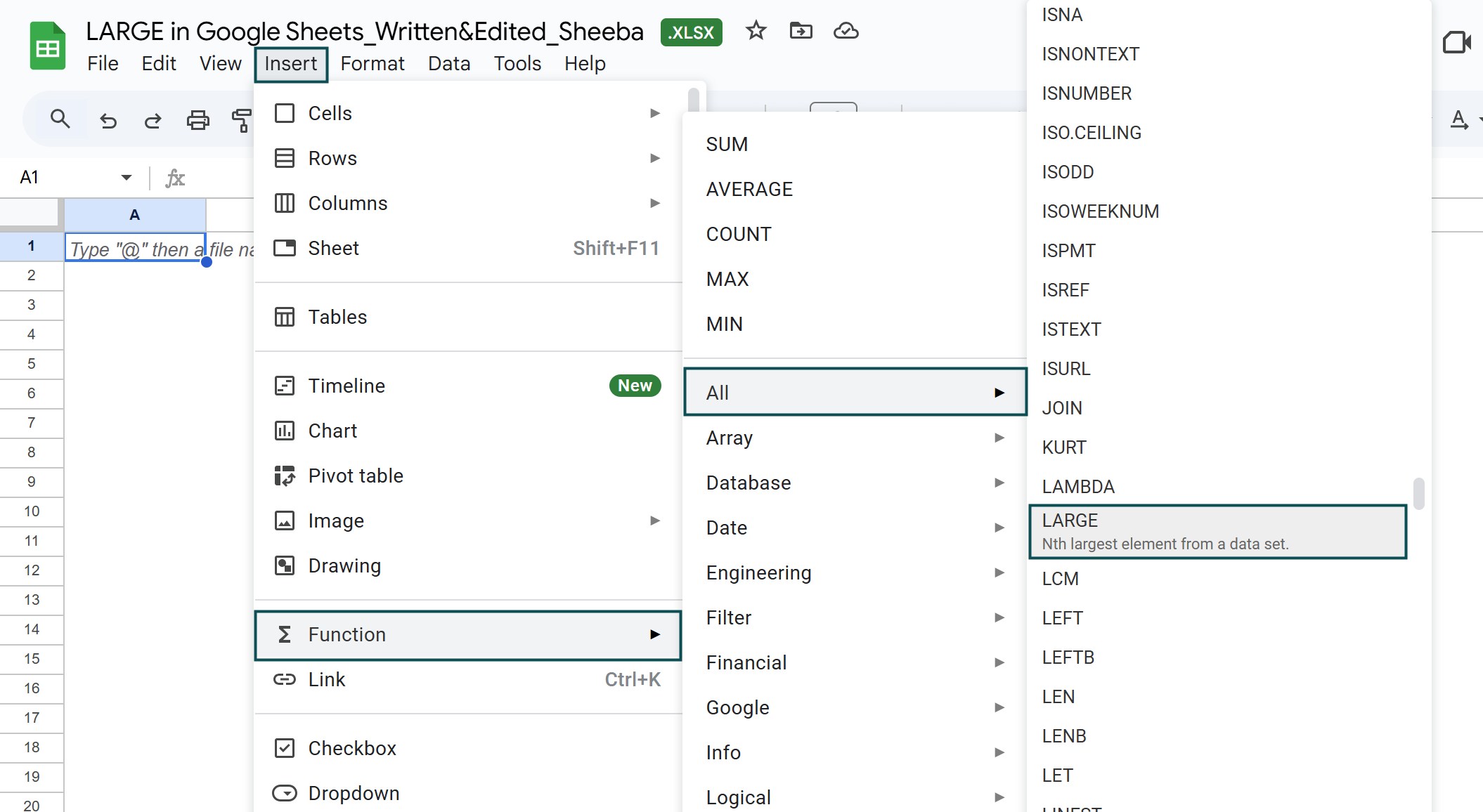
FAQ-2
However, as always, entering the function manually is the best way to avoid confusion.

3. Where else can we find the Google Sheets LARGE function?

Alternatively, we can find the Functions icon to insert the LARGE Google Sheets Function by following the path shown below.
Choose an empty cell – click the “More” option represented by the three vertical dots at the end of the toolbar, as shown below.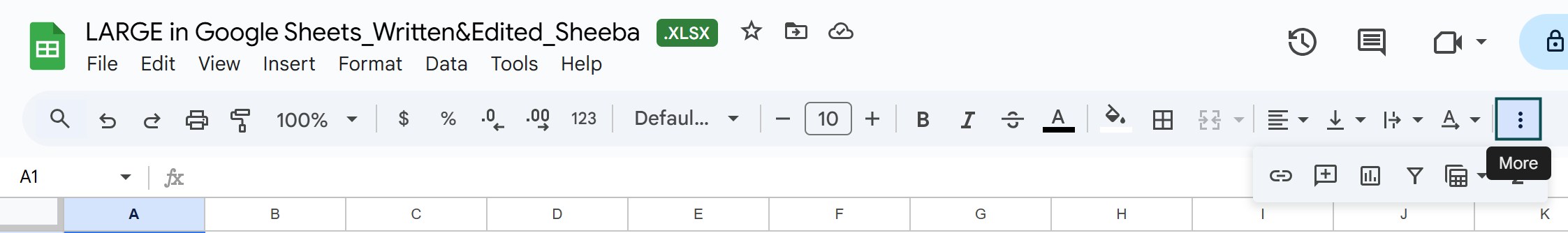
FAQ-3
A list of icons appears when we click the “More” option. Here, click the “Functions” icon, as shown below.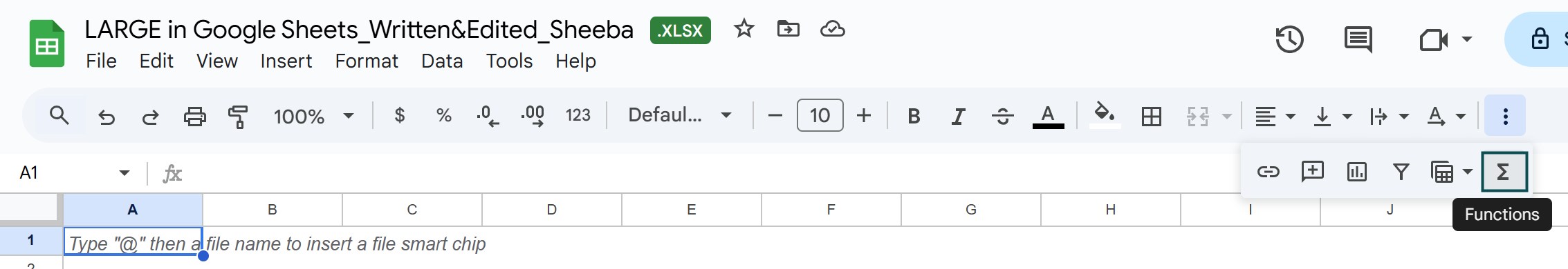
FAQ-3-1
Here, click the “Functions” option – click the “All” option right arrow – select the “LARGE” function, as shown below.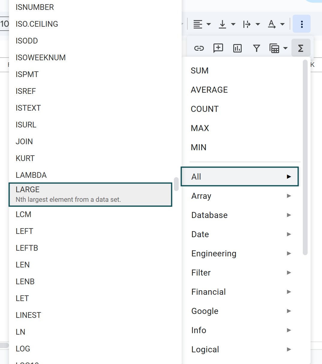
FAQ-3-2

4. What is the way to insert the Google Sheets IF function?

We can insert the Google Sheets IF function as follows:
Choose an empty cell for the output – select the “Insert” tab – click the “Function” option right arrow – click the “Logical” option right arrow – select the “IF” function, as shown below.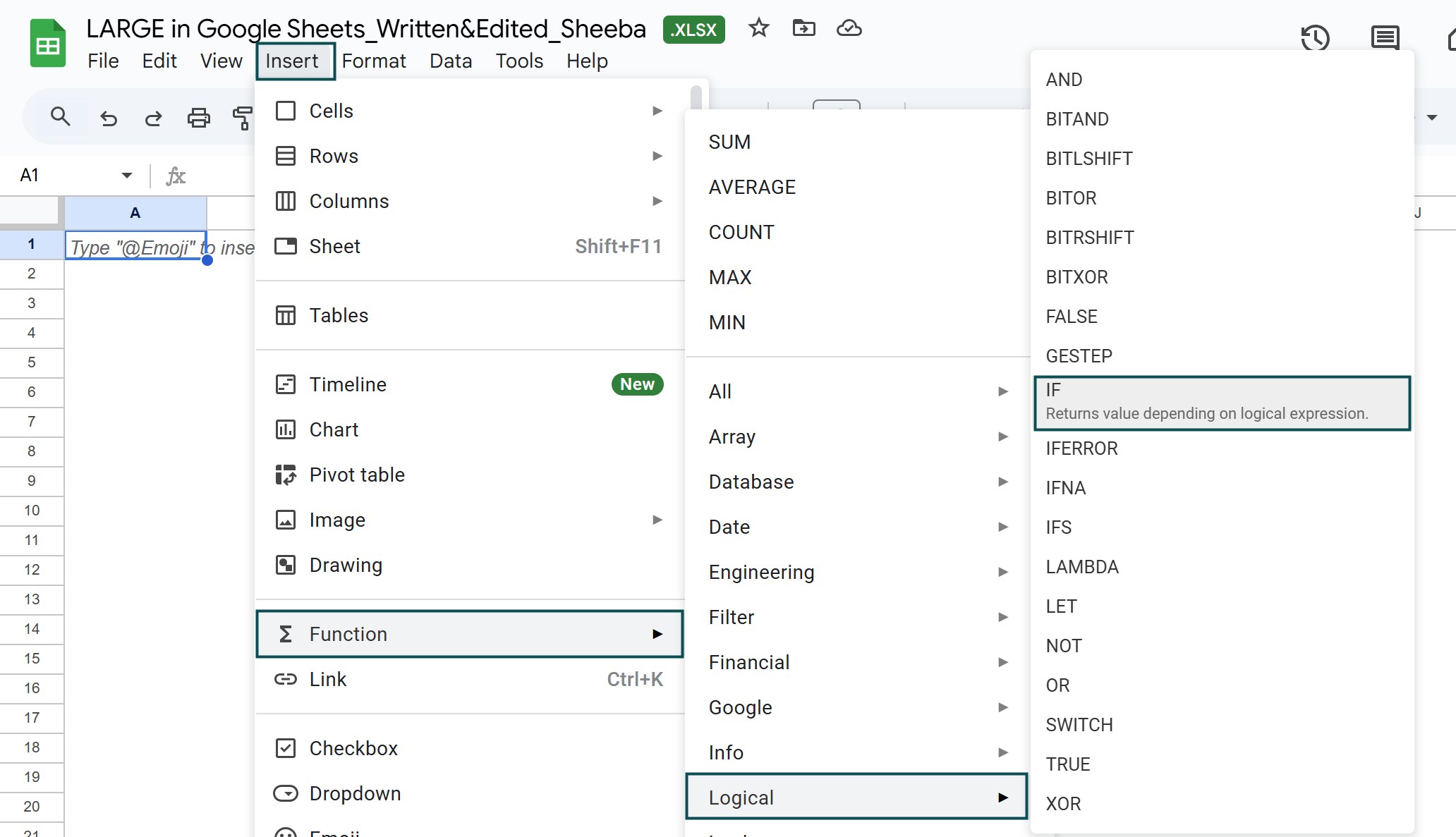
FAQ-4

5. What is the way to insert the Google Sheets FILTER function?

We can insert the Google Sheets FILTER function as follows:
Choose an empty cell for the output – select the “Insert” tab – click the “Function” option right arrow – click the “Filter” option right arrow – select the “FILTER” function, as shown below.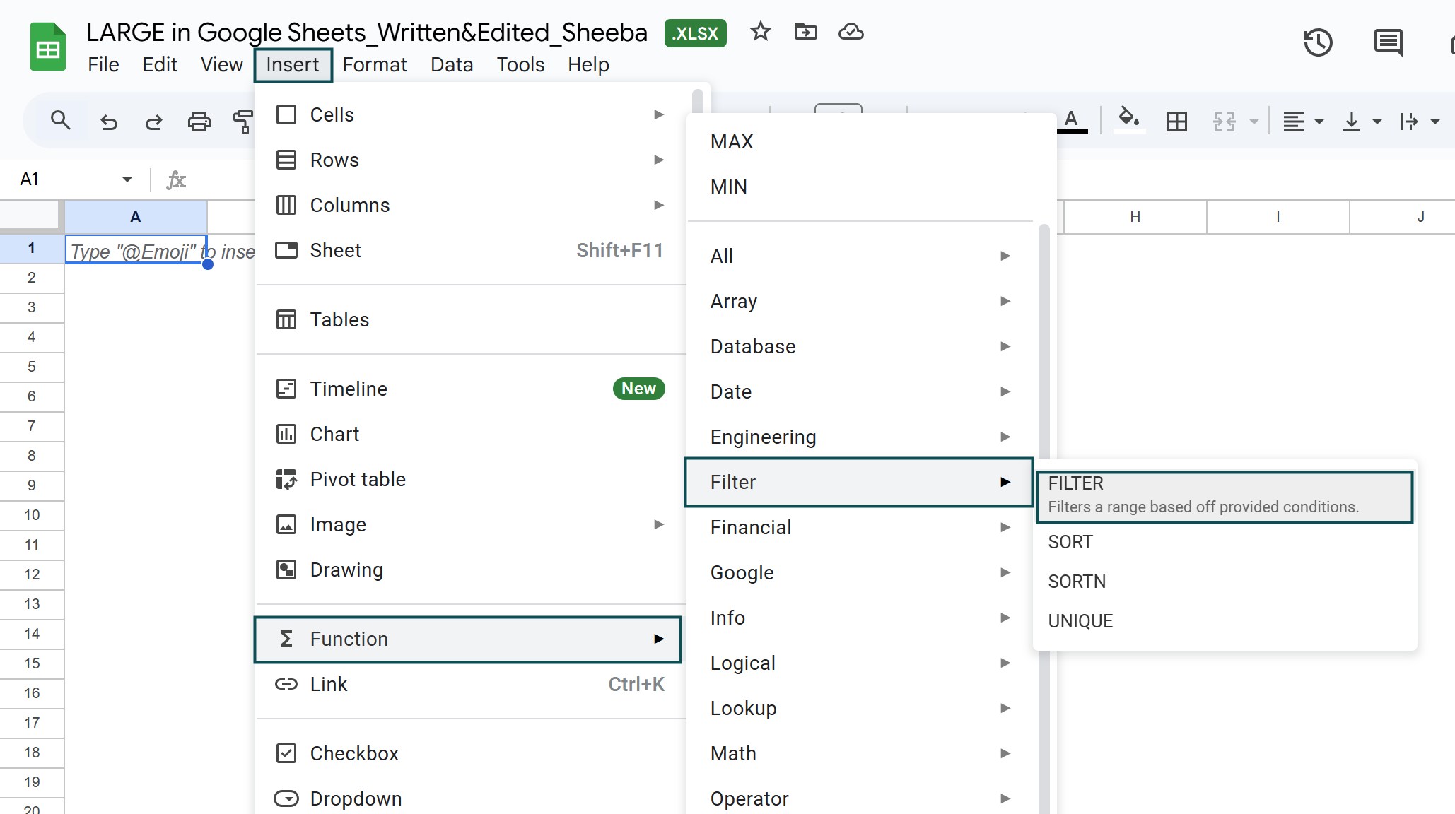
FAQ-5
We can filter the data using the FILTER function, as seen in the above path. The same path can be used to insert the SORT function. However, we can always create a filter and then sort the dataset to organize in ascending or descending order to get the smallest or the largest data in an order, respectively.

Download Template

This article must help understand LARGE In Google Sheets with its formulas and examples. You can download the template here to use it instantly.

LARGE-in-Google-Sheets Download

LARGE In Google Sheets