
What Is LOOKUP Table In Google Sheets?
LOOKUP table in Google sheets, in simple terms, helps users lookup for a value. We can use functions like VLOOKUP, LOOKUP and INDEX-MATCH functions to create a LOOKUP table in Google sheets.
For example, consider the below table showing the list of students and result in column A and B, respectively.

Now, let us learn how to create lookup table using LOOKUP function in Google sheets.
Use this LOOKUP Table In Google Sheets Template to follow along with the examples in this article.
Download Excel TemplateThe steps are:
Step 1: To begin with, select the cell where we want to find the result. In this example, the active cell is E2.
Step 2: Next, we can insert the LOOKUP function formula =LOOKUP(D2,A2:A11,B2:B11)
Step 3: Press Enter key.
We can see the result as shown in the below image.

Likewise, we can use LOOKUP function in Google sheets.
In this article, let us learn how to select the arguments and use the LOOKUP functions with detailed examples in Google sheets.
Key Takeaways
- LOOKUP Table in Google sheets is the data table where users find or look for the value.
- Using LOOKUP table, we can find or look for a specific value from a large dataset in Google sheets with just a few steps.
- Remember, under LOOKUP value, we can use inbuilt functions such as LOOKUP, VLOOKUP, and INDEX-MATCH functions in Google sheets.
- Apart from these functions, we can also use inbuilt functions like IF function to create LOOKUP tables in Google sheets.
How To Create A LOOKUP Table In Google Sheets?
Users can create LOOKUP Table in Google sheets with one of the following three methods. They are:
- Create a Lookup Table Using VLOOKUP Function
- Use LOOKUP Function to Create a LOOKUP Table in Excel
- Use INDEX + MATCH Function
Now, let us learn how to use all the three methods with detailed examples under each method.
#1 -Create A LOOKUP Table Using VLOOKUP Function
We can easily create a LOOKUP table in Google sheets with the help of VLOOKUP function.
The steps are:
- To begin with, insert the table or the data where we want to look for a value.
- In the active cell, where we want to find the result, insert the VLOOKUP formula.
- To insert the formula, simply type =VLOOKUP( and enter the cell references as arguments.
- Press Enter key.
We can find the lookup value immediately.
Now, let us learn how to create a LOOKUP table in Google sheets with an example.
Example #1
For example, consider the below table showing the list of order ID, products, date and status in columns A, B, C and D, respectively.

Now, let us learn how to create a LOOKUP table in Google sheets with the help of VLOOKUP function.
The steps are:
- To begin with, insert the table or the data where we want to look for a value.
- In the active cell, where we want to find the result, insert the VLOOKUP formula.

- Now, select the lookup value present in cell A14 as the first argument.

- Next, select the cell range A2:D11 as the second argument, which is the lookup value.
- Make sure to enter the cell range as absolute reference as shown in the below image.

- Now, enter the number of columns present in the data. In this example, it is 4.

- Finally, we need to enter the logical value, which is TRUE or FALSE as the last argument.

- Press Enter key.
We can find the lookup value immediately as shown in the below image.

Likewise, we can easily create a LOOKUP table in Google sheets with the help of VLOOKUP function.
#2 – Use LOOKUP Function To Create A LOOKUP Table In Google Sheets
Now, let us learn how to use LOOKUP function to create a LOOKUP table in Google sheets.
The steps are:
- To begin with, insert the table or the data where we want to look for a value.
- In the active cell, where we want to find the result, insert the VLOOKUP formula.
- To insert the formula, simply type =LOOKUP( and enter the cell references as arguments.
- Press Enter key.
We can find the lookup value immediately.
Now, let us learn how to create a LOOKUP table in Google sheets with an example.
Example #2
For example, consider the below table showing the list of places and participants in column A and B, respectively.

Now, let us learn how to use LOOKUP function to create a LOOKUP table in Google sheets.
The steps are:
- To begin with, insert the table or the data where we want to look for a value.
- In the active cell, where we want to find the result, insert the LOOKUP formula.

- Now, select the lookup value present in cell A9 as the first argument.

- Next, select the cell range A2:A7,B2:B7 as the second argument, which is the lookup value.

- Close the parenthesis and press Enter key.
We can see the result as shown in the below image.

Likewise, we can easily create a LOOKUP table in Google sheets with the help of LOOKUP function.
#3 – Use INDEX + MATCH Function
Now, let us learn how to use INDEX-MATCH functions to create a LOOKUP table in Google sheets.
The steps are:
- To begin with, insert the table or the data where we want to look for a value.
- In the active cell, where we want to find the result, insert the INDEX-MATCH formulas.
- Enter the cell references as arguments.
- Press Enter key.
We can find the lookup value immediately.
Now, let us learn how to create a LOOKUP table in Google sheets with an example.
Example #3
For example, consider the below table showing the list of fictional characters along with the sales of the products in columns A and B, respectively.

Now, let us learn how to use INDEX-MATCH functions to create a LOOKUP table in Google sheets.
The steps are:
- To begin with, insert the table or the data where we want to look for a value.
- In the active cell, where we want to find the result, insert the INDEX formula.

- Now, select the cell range B2:B6 as the first argument.

- Next, insert the MATCH function as shown in the below image.

- Now, select the lookup value present in cell A8 as the first argument for MATCH function.

- Next, select the cell range A2:A6 as the second argument, as shown in the below image.

- Now, since we want the exact match, i.e., since we want to find the actual lookup value, we need to add 0 as the last argument.

- Close the parenthesis.

- Now, press Enter key.
We can see the result as shown in the below image.

Likewise, we can use INDEX-MATCH functions to create a LOOKUP table in Google sheets.
Important Things To Note
- The LOOKUP functions is an inbuilt category in Google sheets.
- The formula of LOOKUP function in Google sheets is =VLOOKUP(search_key,range,index,[is_sorted])
- The formula of LOOKUP function in Google sheets is =INDEX(return_range,MATCH(search_key,lookup_range,0))
Frequently Asked Questions (FAQs)
Consider the below table showing food products and prices in columns A and B, respectively.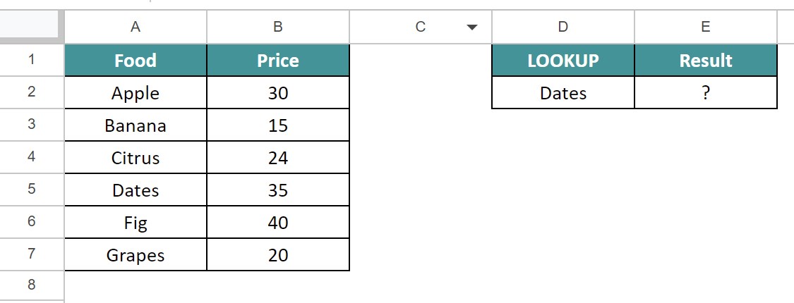
Now, let us learn how to create lookup table using LOOKUP function in Google sheets.
The steps are:
Step 1: To begin with, select the cell where we want to find the result. In this example, the active cell is E2.
Step 2: Next, we can insert the LOOKUP function formula =LOOKUP(D2,A2:A11,B2:B11)
Step 3: Press Enter key.
We can see the result as shown in the below image.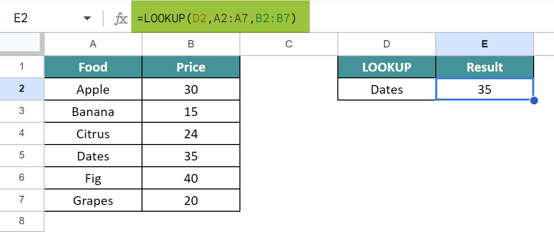
LOOKUP formula in Google sheets is an inbuilt function. We can directly select the desired LOOKUP function under Insert > LOOKUP and desired function.
Or, we can directly type =LOOKUP( in the active cell and select the arguments directly.
Under LOOKUP functions, we have over 16 functions as shown in the below image.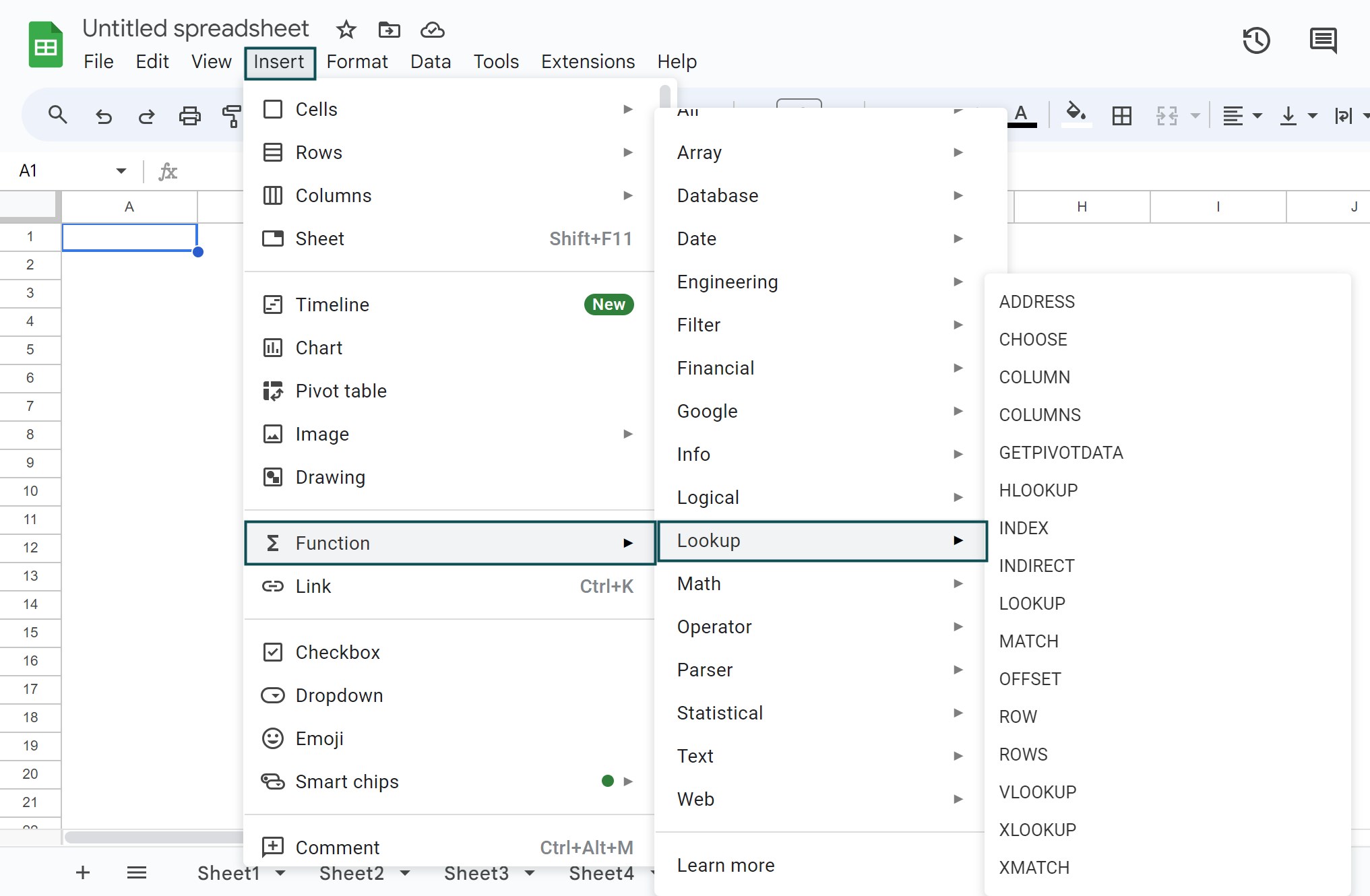
However, the commonly used LOOKUP functions are LOOKUP, VLOOKUP,XLOOKUP, and HLOOKUP functions.
Use this LOOKUP Table In Google Sheets Template to follow along with the examples in this article.
Download Excel Template