
What is a Checklist in Google sheets?
A checklist in Google Sheets is used to track tasks that need to be completed or organized. It allows users to create a list where items can be checked off as they are completed. A check box is a little square box where you click to select or deselect a given option.
If you are creating a Google Sheet checklist, you must make a list of tasks for which the checkboxes will be inserted. Go to Insert -> Checkbox. You will get a checklist, as seen below.
Use this Checklist in Google Sheets Template to follow along with the examples in this article.
Download Excel Template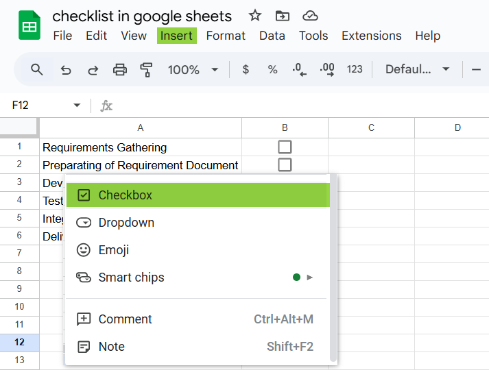
Key Takeaways
- A checklist in Google Sheets is a feature that helps you create interactive checkboxes in your spreadsheet. The checkboxes can be used to monitor tasks and control the display of data.
- A checklist contains a set of checkboxes that can be ticked by users whenever a task is completed.
- You can use conditional formatting to highlight the cells where the checkboxes are selected to monitor task completion.
- To insert a checkbox, go to Insert > Checkbox. The selected cells will now contain checkboxes.
- The main use of checklists is in task management. You can track your tasks and monitor progress.
How to Create a Checklist in Google Sheets?
For starters, Google Sheets is an ideal platform for sharing checklists. It allows you to create, customize, and modify checklists easily. Let us look at how to create checklists as needed in Google Sheets.
- Step 1: Here is a step-by-step guide on how to add a checklist to Google Sheets. First, go to your spreadsheet and choose the list of items you wish to add to your checklist.
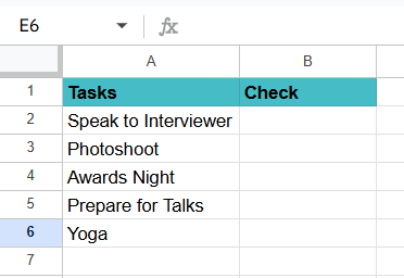
Adding Checklist Items
- Step 2: Select the cells where you want to add the checklist. Add the items one by one.
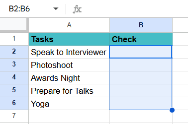
Inserting Checkboxes
- Step 3: Click the “Insert” button on the menu and select “Checkbox” from the drop-down menu.
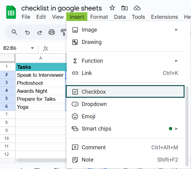
Step 4: Checkboxes will appear in the selected cells. Repeat this step if you add more items want to add to the checklist.
If you want to add additional columns, you can use the “Insert” options in the top navigation menu.
To check or uncheck the items in the checklist, simply click on the checkbox.
Customizing Checklist
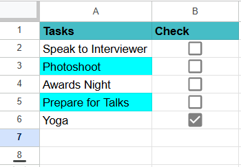
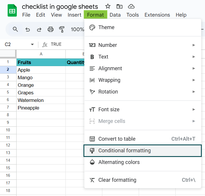
To add a conditional formatting rule, select the cells containing the checkboxes and then click on the “Format” button on the menu. Then, choose “Conditional formatting” from the drop-down menu and select the rule you want to apply.
In this example, we first chose the checklists range and then wished to shade the cells that start with “P.”
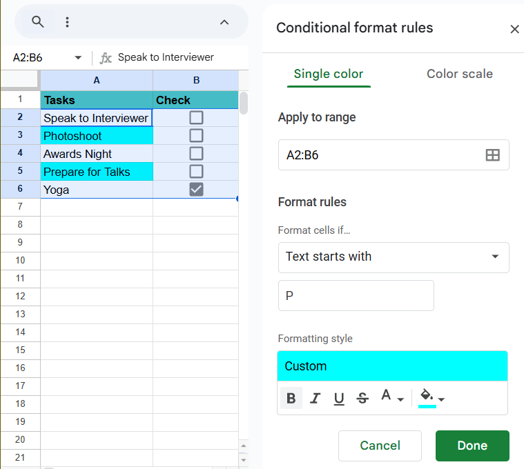
Save the changes to your Google Sheet by clicking on Done, and that’s it!
When you format the list, it looks aesthetically pleasing. You can also customize fonts and colors and insert icons next to each item on the list.
Customization in Google Sheets helps you to personalize your checklist based on preferences. It can be done as follows:
- Add additional columns for additional information.
- Apply conditional formatting to highlight completed tasks automatically.
- Create formulas to track progress.
Examples
When you complete any task on your checklist, you have to click on the corresponding checkbox to mark it as complete so that Google Sheets can update the checkbox status, indicating your progress. Let us look at some examples of how it is done.
Example #1 – Marking Items as Complete
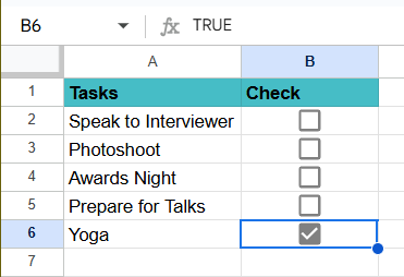
Below is a list of project tasks. Let’s look at how to mark items as complete.
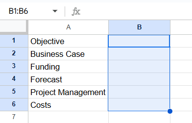
Step 1: To add a checklist, first select the cells to which you wish to add them. Here, we choose B1:B6.
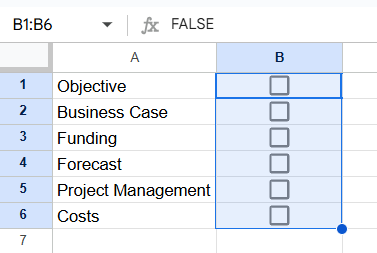
Step 2: Click the “Insert” button on the menu and select “Checkbox” from the drop-down menu. The checkboxes will appear in the selected cells.
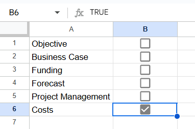
Step 3: When you complete a task on your checklist, you must click on the corresponding checkbox, which is marked as completed. Google Sheets will update the checkbox status, thereby helping you keep track of your progress.
Here, we have marked costs as complete using the checkbox. You can observe that Google Sheets has changed its status from TRUE to FALSE.
Example #2 – Create dynamic charts
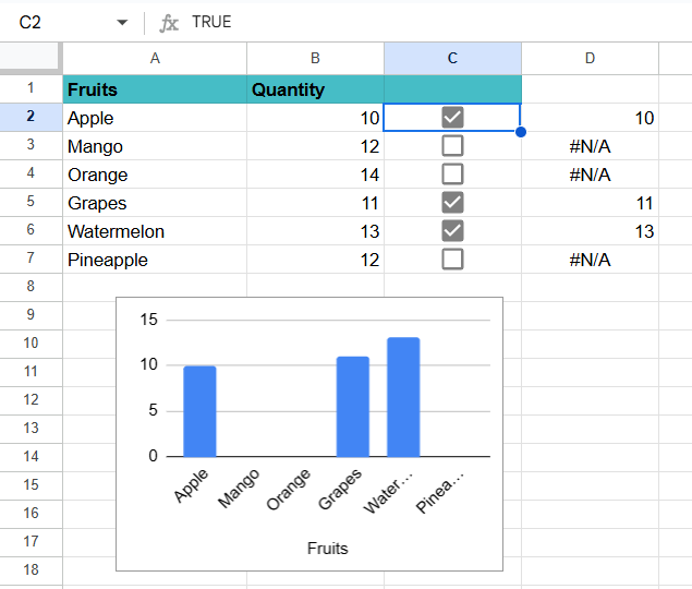
When you wish to create a dynamic chart with checkboxes, Google Sheets allows you to use checkboxes to control what it displays in your chart.
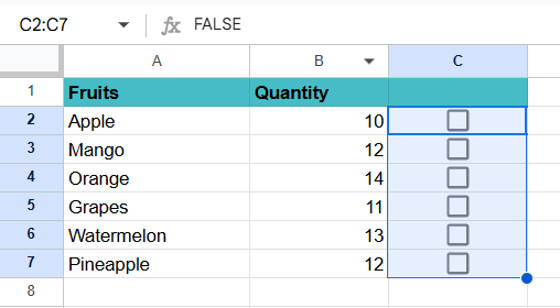
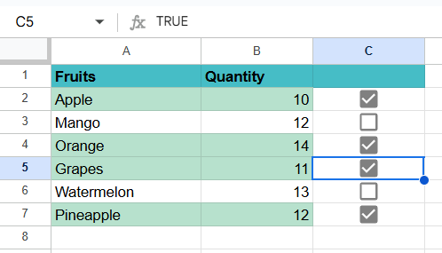
Step 1: We have prepared data regarding some fruits and their quantity available. Let us insert checkboxes for the same.
Go to Insert > Checkbox. It will add checkboxes in the selected cells.
Step 2: Create a dynamic rangein your sheet for dynamic data. For each series, use an IF statement. Use the following in D2 and drag till D7.
=IF(C2, B2, NA())
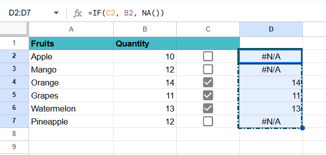
If the checkbox is checked, it returns the value from column B; otherwise, we get #N/A. This output will not be plotted.
Step 3: Now, go to Insert -> Chart. You will get a chart for the checked values.

Step 4: Now, try to select the value for Apple and remove Orange. It updates the chart dynamically.
Example #3 – Using Conditional Formatting for Checklist
Take the same example as above and let us try to add conditional formatting to the checklist.
Step 1: We will add conditional formatting to checked values. Select the range where you wish to apply conditional formatting. Go to Format -> Conditional Formatting.
Step 2: Enter the Google Sheets checkbox formula which we used for the chart.
=IF(C2,B2,NA()) in the Format Rules box. Press Done.
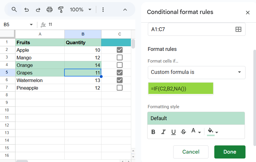
You can see that it highlights the cells of the checkboxes that are checked.
When you check different boxes, the highlighting changes accordingly.
This setup allows you to visualize the checklist based on your selections dynamically.
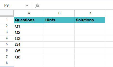
Example #4 – Show/hide hints and solutions to a test
It is a fascinating example. Some students take an exam. We have solutions and hints to the six questions that appear for the test.
Step 1: The table is as follows.
Step 2: In Column D, we can add the checkboxes for hints. Select D2 to D7. Go to Insert -> Checkbox. You get it as shown below.
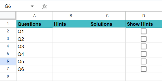
Similarly, we can do the same in Column E for the solutions.
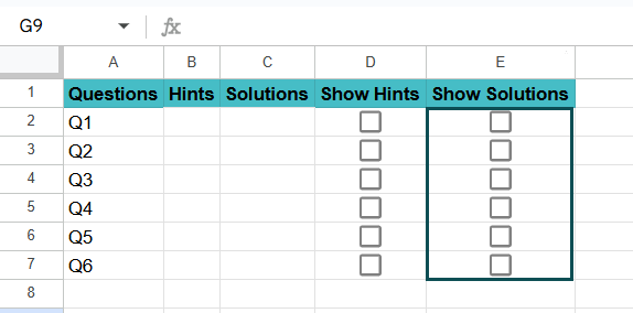
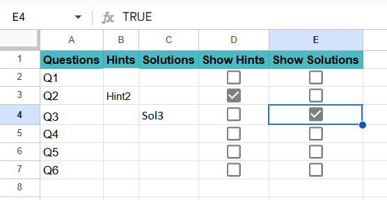
Step 3: Our aim is that when a student selects a particular checkbox, say E4, the solution for the third question will be unveiled.
If he selects D5, it unveils the hint for the fourth question.
Use the following formula in B2.
=IF(D2,”Hint”&1,””). Press Enter.
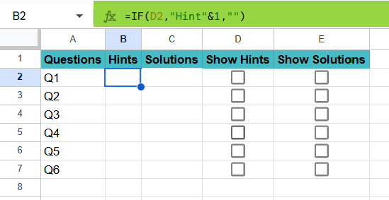
This formula will print Hint1 in cell B2 one ticks the checkbox in D2; otherwise, it will show a blank.
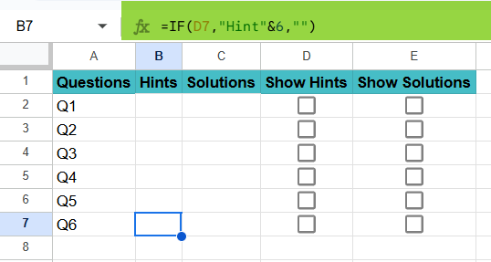
Step 4: Copy-paste the formula till B7, change the hint numbers alone as =IF(D3,”Hint”&2,””), =IF(D3,”Hint”&3,””), etc.
Step 5: Now, we repeat the same steps to display the solution. Paste the formula
=IF(E2,”Sol”&1,””) in cell C2 and drag it till C7 changing only the number as =IF(E2,”Sol”&2,””), =IF(E2,”Sol”&3,””), etc.

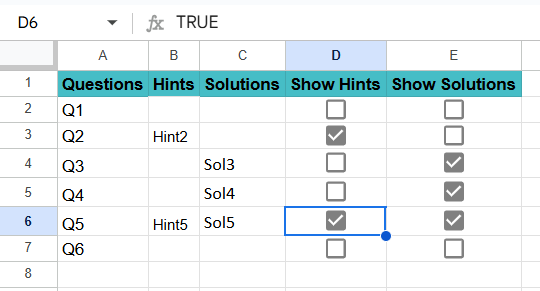
Step 6: Now, let us tick D3 and E4. Observe what happens. The hint for Q2 and the solution for Q3 are displayed.
This can be used for other questions. Select the appropriate box depending on whether you need a hint or solution!
Important Things To Note
- You can count the checked boxes using the COUNTIF function.
- You can create a checklist using data validation by going to Data > Data Validation and then setting a list of items and allowing users to select options.
- You can use formulas to show or hide information, as in Example 4, to hide or show hints/solutions.
Frequently Asked Questions (FAQs)
Checklists are handy to track the progress of tasks. Their main uses include:
Task Management: They help in organizing tasks, making it simple to track the progress of projects or assignments.
Interactive: These checklists are interactive and can be used to check or uncheck items directly in the sheet.
Personalize: You can personalize your checklist to suit your needs by adding dates, priorities, etc.
Sharing: Google Sheets is versatile; hence, you can share your checklist with multiple users at the same time.
Formulas: You can add formulas to perform calculations within your checklist.
Conditional Formatting: Using your checklist, you can highlight specific cells based on certain conditions to see the progress of your tasks.
To insert a checklist,
• Select the cell(s) to insert the checklist.
• Go to Insert > Checkbox.
You get checkboxes in the selected cells.
You can use an IF statement to link a checkbox to a formula. For example, you can use =IF(A1, “Checked”, “Unchecked”), where the formula will return “Checked” if the checkbox in A1 is selected.
If you’re working on a checklist with a team, Google Sheets’ collaborative feature makes it easy to share the checklist. Your team members can view or edit the checklist in real-time when you share it. To share the checklist, you should click on the “Share” button in the top-right corner of Google Sheets and enter the email Ids of the people you want to share it with. You can also specify access levels.
Use this Checklist in Google Sheets Template to follow along with the examples in this article.
Download Excel Template