
What is MROUND Function in Google Sheets?
The MROUND function in Google Sheets rounds a number to the nearest multiple of a specified factor. This function is useful for applications where you need to round up a number to the nearest whole number, nearest 0.5, and so on. You can use MROUND to make your data look professional.
Rounding is done when, after dividing the value by factor, the remainder is greater than or equal to half the value of the factor. In case the value is an exact multiple, no rounding occurs. Let us look at an example. Let us use the formula below to round up the value PI to 0.05:
Enter the following function in an empty cell =MROUND(PI(), 0.05). The number will be rounded up to 3.15.

Use this MROUND in Google Sheets Template to follow along with the examples in this article.
Download Excel TemplateKey Takeaways
- The MROUND function in Google Sheets rounds a number to the nearest multiple of a specified factor. It’s particularly helpful for rounding numbers to a specific increment. Common uses include rounding prices to the nearest dollar, rounding measurements to the nearest tenth, adjusting times to the nearest 15 minutes and so on.
- The syntax of MROUND is as follows:
- =MROUND(number, multiple)
- number: The number you want to round.
- multiple: The multiple to which you want to round the number.
- If the number is already a multiple of the specified multiple, MROUND returns the original value itself.
- If the specified multiple is negative, the number should also be a negative value.
- Its key uses include rounding in tax calculation and in rounding up the cost of items.
Syntax
The syntax of the MROUND function in Google Sheets is as follows:
=MROUND(value, multiple)
- value – The number you want to round
- multiple – The multiple to which you want to round up.
If “multiple” is a negative number, “value” should also be negative. They must both be positive or both negative. If either is zero, MROUND will return 0.
How to use MROUND Function in Google Sheets?
There are two ways to enter the MROUND function in Google Sheets.
Entering the MROUND Function manually
Let us look at a simple way to manually round some numbers to some factors. We have entered the numbers and the corresponding factors we want to round them to in Column A.

Step 1: In cell B2, enter the following formula with the open braces.
=MROUND(

Step 2: To round the numbers to the corresponding factors, use the following arguments: =MROUND(A2, B2) and close the parenthesis.

Step 3: Press Enter. Drag the formula down to the other cells in the column to apply it to all the values in the range.

You can observe how the numbers have been rounded to the nearest multiple.
Using the Google Menu bar
- We can also enter the same function using the Google Menu bar.
- Go to the menu bar and click on “Insert” ➝ “Function” ➝ “Math” ➝ “MROUND.”
- Enter the required arguments. Close the bracket and press the “Enter” key.

Note: If the value argument is equidistant from the two multiples of the factor, the multiple with the greater absolute value will be returned. For example, =MROUND(7.5,5) rounds to 10.
Examples
Now that we have understood some of the nitty-gritties of the function, let’s look at some interesting examples.
Example #1 – Rounding Prices
Imagine you have some sales data with plenty of decimal points. To give a neater look and aid in more accurate calculations, you must round the numbers up to the nearest tenth of a dollar to plan inventory.
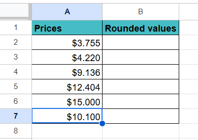
Step 1: The following are the sales figures which should be rounded.
Step 2: Now, round the figures to one-tenth of a dollar and highlight those sales less than $10.
Use the MROUND formula in Google Sheets in cell B2 as follows.
=MROUND(A2, 0.1)
Press Enter.

Step 3: To get the values for the other cells, drag the formula to B7.

Step 4: To highlight the cells with values below $10, go to Format -> Conditional Formatting.
In the Conditional Format rules pane on the right, select the range as B1:B8, choose Less than under Format rules, and enter 10.

Step 6: Press Done.

Explanation of result:
If the value is 3.755, the MROUND function converts the total sales to $4 for a factor of 0.1.
For instance, it rounds $10.1 to $11.
$9.136 is rounded to $10 for a 0.1 factor.
Example #2 – Rounding to the Nearest Quarter
We have a list of test scores in Google Sheets. The teacher wants to round the percentages to the nearest 0.25 for grading. MROUND can save you time and ensure consistency.
Step 1: Suppose you have the following scores of students in cells A1 to A7.

Step 2: Now, we use the MROUND function in B2 to round the scores to the nearest 0.25.
=MROUND(A2, 0.25).

Step 3: Now, drag the formula down from cell B1 to B7 to apply the formula to the other scores.

Step 4: It rounds all the scores to the nearest 0.25 factor.
It rounds each score in column A to the nearest 0.25 in column B. As seen, 98.657 becomes 98.75, and even 67.89 becomes 68.
91.1 gets rounded to the nearest 0.25 at 91. So, as seen, 95.555 becomes 95.5. 75 while 90.1 becomes 90.
Example #3 – Using MROUND with IF function
Let’s have a list of scores again. If the score is greater than 50, we wish to round the price to the nearest 0.50, or keep it as it is if it is less than 50.
You can use the MROUND function with the IF function to achieve this.

Step 1: Use the following formula in cell B2.
=IF(A2 > 50, MROUND(A2, 0.5), A2). Press Enter.
Here, we check if the score is above 50. If so, we round the score to the nearest 0.5. Else, we display the same value.

Step 2: Drag the formula till cell B8.

Important Things to Note
- The two arguments of the MROUND function must have the same sign, they must both be positive or negative. If they do not have the same sign, you get the #NUM error. If any of them are zero, MROUND will return 0.
- You can use MROUND with ARRAYFORMULA to apply the function to a range of cells simultaneously. MROUND is wrapped around ARRAYFORMULA as shown in the following example.
- =ARRAYFORMULA(MROUND(A1:A5, 5))
- To use MROUND in Google Sheets to round values to the closest half-hour, you can enter a half hour which is the multiple argument as “0:30” or “0:30:00.“
- You can combine MROUND with other functions like SUM, AVERAGE, or IF to create more complex formulas.
Frequently Asked Questions (FAQs)
1. Businesses use it to round prices to the nearest dollar or specific currency value to standardize the pricing of their products.
2. It is helpful if you have to round time entries by a specific increment, like rounding to the nearest 5 minutes.
3. In finance, rounding to the nearest decimal value, such as tens or hundreds, simplifies understanding of reports and presentations.
Google Sheets offers many different functions for rounding values. Let’s look at a few.
1. ROUND: The ROUND function rounds a number to a certain number of decimal places. It rounds up when the decimal place is greater than or equal to 5. Otherwise, it rounds down.
2. ROUNDDOWN: The ROUNDDOWN function rounds down a number to a certain number of decimal places. For instance, it rounds 5.7 to 5.
3. FLOOR: It rounds a number down to the nearest integer multiple of the mentioned significance. For instance, =FLOOR(1.27, 0.05) gives a result 1.25
4. CEILING: The CEILING function is the opposite of FLOOR and rounds a number up to the nearest integer multiple of the mentioned significance. Here, =CEILING(1.27, 0.05) gives a result of 1.30.
We can use MROUND in conditional formatting to highlight cells that have been rounded with specific multiples. The steps are listed below.
• Select the cells you wish to format.
• As the next step, go to Format -> Conditional formatting. Go to the next step.
• Under Format cells if, select Custom formula is and enter the following formula as an example. =MROUND(A1, 10) = A1. It is for highlighting cell values that are multiples of 10.
• Choose the required changes, such as background color or bold text. Press Done.
This helps you visualize the values which are multiples of 10 in the data with ease.
Use this MROUND in Google Sheets Template to follow along with the examples in this article.
Download Excel Template