
What Is Not Equal To In Google Sheets?
The Not Equal To in Google Sheets is a feature to compare two values and check if they are equal or similar to each other or not. The Sign or Symbol for Not Equal to is “<>”. The Google Sheets Not Equal To returns the logical values as TRUE, if the compared values vary or are not equal and FALSE, if the compared values are the same or equal.
For example, we will compare the values given below using the Not Equal To in Google Sheets.
Use this Not Equal To In Google Sheets Template to follow along with the examples in this article.
Download Excel Template
Select cell C2, enter the formula =A2<>B2, press “Enter” and drag the formula from cell C2 to C5 using the fill handle, as shown below.

As shown above, the output is TRUE in cells C2, C4 and C5, because the values are different from the compared values. However, cell C3 is FALSE as the compared value is the same.
Key Takeaways
- The Not Equal To in Google Sheets checks whether the values getting compared, regardless of the nature whether they are numerical or text, are similar or not.
- The function always requires two values to check. While comparing values, if one of the values is a blank cell, we will get the output as “True”. And if both the cells are blank, we get the output as “False”. These are a few scenarios of the Boolean default values.
- We can use conditional functions such as the IF, COUNTIF andthe SUMIF to get an alternate output instead of the default “True” or “False”.
- To use this feature we can use a value and the other value to compare can be entered within the formula as well, like “cell reference of a value<>200” or “abc<>cell reference of value”.
Syntax
- Google Sheets does not have an inbuilt function for “Not Equal To”. We can build the formula as “=value1<>value2”, where Value1 and Value2 are the cell references or the values which must be entered within double-quotes.
- The Symbol For “Not Equal To” in Google Sheets is “<>”, i.e. the less than symbol “<” and the greater than symbol “>” facing each other].
How To Use “Not Equal To” Function In Google Sheets?
We can use the “Not Equal To” in Google Sheets as follows:
Step 1: Enter the “Equal To” (=) sign to start the formula.
Step 2: Select the first value as cell references. Else enter a direct value within double-quotes.
Step 3: Then, type the “Not Equal To” sign, i.e.,<>.
Step 4: Select the second value as cell references or direct value within double-quotes.
The syntax will look as shown below,

Step 5: Finally, press “Enter” to view the results.
Examples
We will consider some Not Equal To in Google Sheets Examples to compare numeric and textual values, also use this feature along with some conditional functions such as IF(), COUNTIF() and SUMIF().
Example #1 – Compare Two Numeric Values-
The following table consists of numeric values and we will compare the values to check if they are equal or not using the Not Equal To in Google Sheets.

The steps to use the Not Equal To function in Google Sheets are as follows:
Step 1: Select cell C2 and enter the formula =A2<>B2, as shown below.

Step 2: Press “Enter”. We get the results shown below.
[Note: Google sheets provide an autofill option for results. We can choose it or use the autofill option.]

Step 3: Drag the formula from cell C2 to C6 using the fill handle, to get the following results.

Example #2 – Compare Two Text Values –
The table below consists of textual values and we will compare them to check if they are equal or not using the Not Equal To in Google Sheets.

The steps to use the Not Equal To function in Google Sheets are as follows:
Step 1: Select cell C2, enter the formula =A2<>B2 and press “Enter”, as shown below.

Step 2: Check/tick the Auto Fill option, to get the following results

We see that the Not Equal To feature is not case-sensitive. Therefore, regardless of the case or the font style of the letters, if they are same, they are equal or not.
Example #3 – IF Function With “Not Equal To” Condition –
We willcompare the given valuesusing the IF Function with the Not Equal To in Google Sheets and return alternate results other than the default, True or False.

The steps to compare cells using the IF function and the Google Sheets Not Equal To are as follows:
Step 1: Select cell C2 and enter the formula =IF(B2<>”No”,”Sale”,”No Stock”), as shown below.

Step 2: Drag the formula from cell C2 to C6 using the fill handle, to get the following results.

Example #4 – COUNTIF Function With “Not Equal To” Condition –
We willcompare the given valuesusing the COUNTIF Function with the Not Equal To in Google Sheets to find the count of values that satisfy the given criteria.

- The COUNTIF function is from the COUNT function familyin Google Sheets, like the COUNTA and COUNTBLANK functions. It is a pre-defined function in Google Sheets that counts all the cells in the range as specified by the conditions.
- The formula of the COUNTIF function is, =COUNTIF(range,criteria)
The steps tocompare valuesusing the COUNTIF() withthe Google Sheets Not Equal To are,
Step 1: Select cell E2, enter the formula =COUNTIF(B2:B11,”<>HR”), as shown below.

Step 2: Press “Enter” to get the output, as shown below.

We get the output as 8, because out of the 10 values there are 8 values that satisfy the condition that it must be not equal to “HR”.
Example #5 – SUMIF Function With “Not Equal To” Condition –
We willcompare the given valuesusing the SUMIF Function with the Not Equal To in Google Sheets to find the total of the values that satisfy the given criteria.

- The SUMIF function is from the SUM function familyin Google Sheets, like the SUM and SUMPRODUCT functions. It is a pre-defined function in Google Sheets that adds all the cells in the range as specified by the conditions.
- The formula of the SUMIF function is, =SUMIF(range,criteria,[sum_range])
The steps tocompare valuesusing the SUMIF() withthe Google Sheets Not Equal To feature are,
Step 1: Select cell B11 and enter the formula =SUMIF(A2:A8,”<>Toiletries”,B2:B8), as shown below.

Step 2: Press “Enter” to get the output, as shown below.

We get the output as shown above, as the values that satisfy the condition are totalled.
Important Things To Note
- The sign or Symbol for Not Equal to is ≠, however, in Google Sheets, we use “<>” symbol.[The less than symbol “<” and the greater than symbol “>” facing each other].
- The Not Equal to in Google Sheets is case-insensitive. So, whether the strings compared are uppercase, lowercase, or a combination of both, the function will return accurate results.
- We can also compare a numeric value with a text value, as shown below. The output will be “True”, implying that the two values are different.
Frequently Asked Questions (FAQs)
A few reasons the Not Equal To in Google Sheets do not work are,
a. We have entered the Not Equal To symbol incorrectly.
b. While entering the conditional function we have not entered the condition with the Not Equal To symbol within double-quotes.
c. The arguments are entered as direct values without double-quotes.
We can insert the COUNTIFS function in Google Sheets as follows:
Choose an empty cell for the output 🡪 select the “Insert” tab 🡪click the “Function” option right arrow 🡪 click the “Math” option right arrow 🡪 select the “COUNTIFS” function, as shown below.
The “COUNTIFS” formulaappears, as shown below. Enter the argument as the cell reference.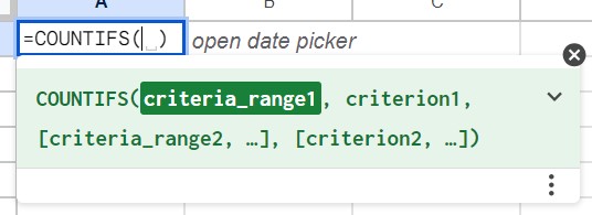
We can use the same path to select other COUNT functions such as COUNTBLANK(), COUNTIF(), COUNTIFS() and COUNTUNIQUE().
We can insert the SUMIF function in Google Sheets as follows:
Choose an empty cell for output 🡪 select the “Insert” tab 🡪 click the “Function” option right arrow 🡪 click the “Math” option right arrow 🡪 select the “SUMIF” function, as shown below.
The SUMIF formula appears as shown below. 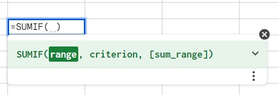
We can use the same path to select other SUM functions such as SUM(), SUMIF() and SUMIFS().
Use this Not Equal To In Google Sheets Template to follow along with the examples in this article.
Download Excel Template