
What Is Daverage Google Sheets?
Daverage in Google sheets, is just like AVERAGE function formula in Google sheets. The daverage function gives the average of values with a specific criteria or condition whereas, there is no condition in the AVERAGE function.
The ‘d’ in the daverage function stands for database. So, we can also call daverage function as database average function in Google sheets.
Use this Daverage Google Sheets Template to follow along with the examples in this article.
Download Excel TemplateFor example, consider the below table showing customer, product, quantity in columns A,B and C, respectively.

Now, the condition to use in the daverage formula is ‘Dates’. It is available in the cell range E1:E2. Let us learn how to calculate daverage function in Google sheets.
To begin with, select the cell F2 and insert the formula =DAVERAGE(A1:C9,C1,E1:E2) and press Enter key.
We will be able to see the daverage result in cell F2, as shown in the below image.

Likewise, we can use daverage function in Google sheets to find the result.
In this article, let us learn how to use daverage function in Google sheets with detailed examples.
Key Takeaways
- daverage function in Google sheets is similar to the AVERAGE function in Google sheets but uses condition or criteria.
- The ‘d’ in the daverage function stands for database average function.
- Formula of daverage Google sheets function is =DAVERAGE(database,field,criteria) where all three arguments are mandatory.
- database is the data range used to find the daverage
- field is the column with numeric values or text values. It can also be a column index
- criteria is the range showing condition used to filter the data
- We can use daverage function with single criteria and multiple criteria, or even without criteria.
Daverage() Google Sheets Formula

The formula or syntax of daverage Google sheets formula is =DAVERAGE(database,field,criteria)
where,
- database is the data range having labels in the first row
- field is the data with numeric values. Remember, this can also have text or be a column index
- criteria is the range with condition that is used to filter the data
All three arguments are mandatory.
How To Use Daverage Function In Google Sheets ?
We can use daverage function in Google sheets with two methods. They are:
- Selecting the formula under Insert tab
- Manually typing the formula
Method #1 – Selecting the formula under Insert tab
The steps are:
Step 1: To begin with, we need to insert the data. Select the cell where we want to find the result.
Step 2: Next, click on Insert Tab. Then select Function option.

Step 3: Now, in the list of options, select Database and click on DAVAERAGE function.

We will be able to see the function in Google sheets. Now, select the arguments and press Enter key to find the result.
Method #2 – Manually typing the formula
Step 1: To begin with, we need to insert the data. Select the cell where we want to find the result.
Step 2: Enter =DAVERAGE or =dav. Then select the daverage function in the list of options.

Step 3: We will be able to see the function in Google sheets. Now, select the arguments.
Step 4: Press Enter key to find the result.
Likewise, we can use one of the two arguments to use daverage function in Google sheets.
Examples
Let us learn how to use daverage function in Google sheets with detailed examples.
Example #1 – DAVERAGE With Single Criteria
For example, consider the below table showing date, product and quantity in columns A, B and C, respectively. The single criteria or condition to be used to filter and find the average is available in the cell range E1:E2.

Now, let us learn how to calculate daverage function in Google sheets.
The steps are:
Step 1: To begin with, insert the data in Google sheets. In this example, the data is available in the cell range A1:C9. Next, we need to select the cell where we want to find the result. In this example, we need to select the cell F2.
Step 2: Next, insert the DAVERAGE Google sheets function formula.
So, the complete formula is =DAVERAGE(A1:C9,”Quantity”,E1:E2).

Step 3: Press Enter key.
We will be able to see the daverage result in cell F2, as shown in the below image.

Likewise, we can use daverage function in Google sheets to find the result with single criteria.
Example #2 – DAVERAGE Without Criteria
For better understanding, let us use the same example we used in example #1. Consider the below table showing date, product and quantity in columns A, B and C, respectively. In this example, let us find daverage without criteria.

Now, let us learn how to calculate daverage function.
The steps are:
Step 1: To begin with, insert the data in Google sheets. In this example, the data is available in the cell range A1:C9. Next, we need to select the cell where we want to find the result. In this example, we need to select the cell F2.
Step 2: Next, insert the DAVERAGE Google sheets function formula.
So, the complete formula is =DAVERAGE(A1:C9,”Quantity”,E1:E2).

Step 3: Press Enter key.
We will be able to see the daverage result in cell F2, as shown in the below image.

Likewise, we can use daverage function to find the result without criteria.
Example #3 – DAVERAGE With Multiple Criteria
For example, consider the below table showing date, name, region and projects in columns A, B, C and D, respectively. The multiple criteria or condition to be used to filter and find the average is available in the cell range F1:F2.

Now, let us learn how to calculate daverage function.
The steps are:
Step 1: To begin with, insert the data in Google sheets. In this example, the data is available in the cell range A1:D13. Next, we need to select the cell where we want to find the result. In this example, we need to select the cell G2.
Step 2: Next, insert the DAVERAGE Google sheets function formula.
So, the complete formula is =DAVERAGE(B1:D13,”Projects”,F1:F3)

Step 3: Press Enter key.
We will be able to see the daverage result in cell G2, as shown in the below image.

Likewise, we can use daverage function to find the result without criteria.
Example #4 – Comparison Operators In Google Sheets
For example, consider the below table showing name, region and projects in columns A, B and C, respectively. We can see the comparison criteria in data condition in cell E2.

Now, let us learn how to calculate daverage function with comparison operator.
The steps are:
Step 1: To begin with, insert the data in Google sheets. In this example, the data is available in the cell range A1:D13. Next, we need to select the cell where we want to find the result. In this example, we need to select the cell G2.
Step 2: Next, insert the DAVERAGE Google sheets function formula.
So, the complete formula is =DAVERAGE(A1:D13,”Projects”,E1:F2)

Step 3: Press Enter key.
We will be able to see the daverage result in cell G2, as shown in the below image.

Likewise, we can use daverage function to find the result using comparison operators.
Important Things To Note
- DAVERAGE function in Google sheets is database average function.
- It is used to find the average with the condition or criteria.
- Similar to using IF function with logical operators, we can use daverage function with comparison operators.
Frequently Asked Questions (FAQs)
For example, consider the below table showing date, product and quantity in columns A, B and C, respectively. The single criteria or condition to be used to filter and find the average is available in the cell range E1:E2.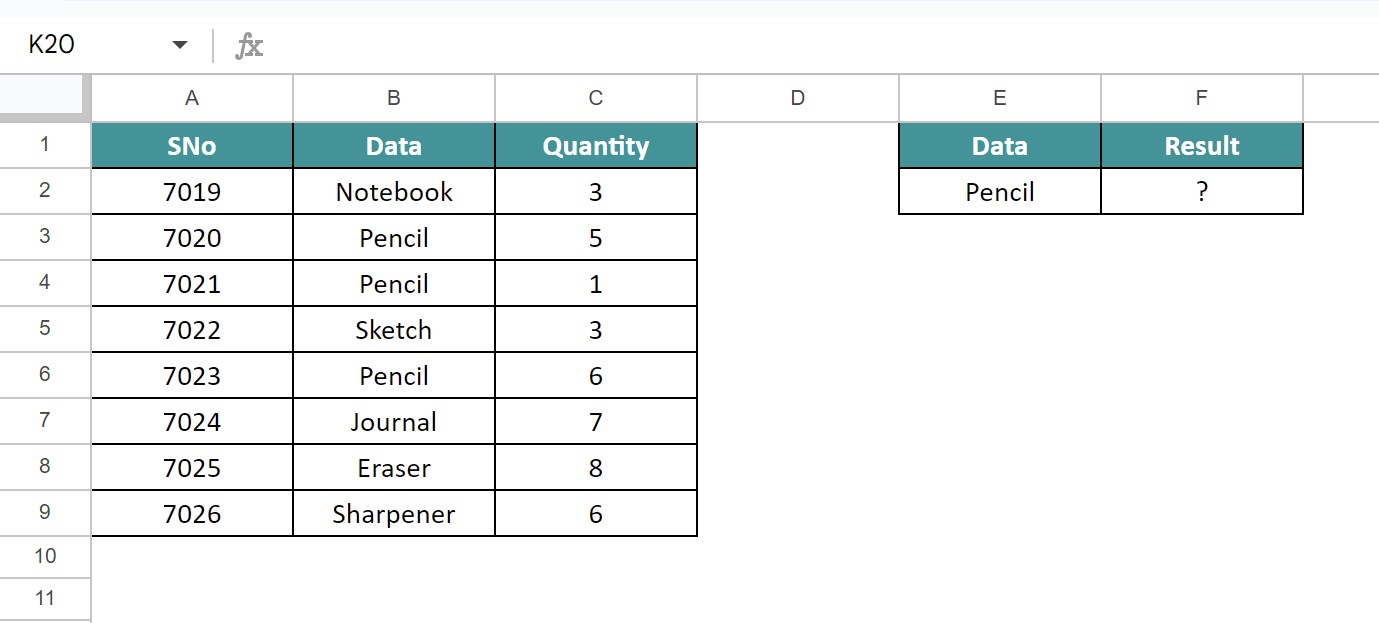
Now, let us learn how to calculate daverage function.
The steps are:
Step 1: To begin with, insert the data in Google sheets. In this example, the data is available in the cell range A1:C9. Next, we need to select the cell where we want to find the result. In this example, we need to select the cell F2.
Step 2: Next, insert the DAVERAGE Google sheets function formula.
So, the complete formula is =DAVERAGE(A1:C9,”Quantity”,E1:E2)
Step 3: Press Enter key.
We will be able to see the daverage result in cell F2, as shown in the below image.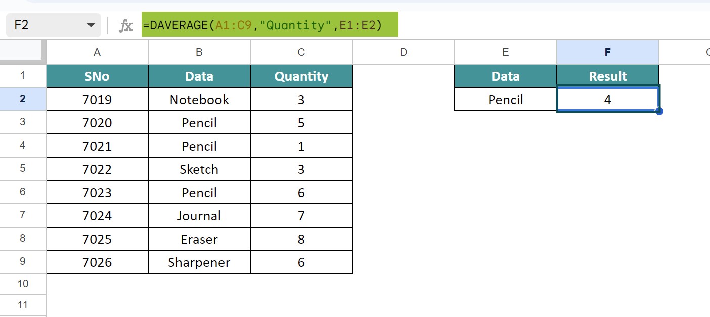
Likewise, we can use daverage function to find the result.
Daverage function may not work if,
• The condition we use in the criteria is in par with the data included in the database.
• Similarly, daverage function will not work if the field is not related with the database.
The daverage function is similar to the AVERAGEIF function and we can find the average of data with a criteria or condition. In case there are multiple conditions, we can also use AVERAGEIFS function in Google sheets.
Use this Daverage Google Sheets Template to follow along with the examples in this article.
Download Excel TemplateRecommended Articles
Continue with these related resources when you want the next practical step in this topic.
- MATH Functions In Google Sheets
- SUM Google Sheets Function
- AUTOSUM In Google Sheets
- COUNT FUNCTION IN GOOGLE SHEETS
- AVERAGE In Google Sheets
Explore the full Google Sheets Math Functions guide or browse Google Sheets Resources.