
What is TRUE Function in Google Sheets?
The TRUE function in Google Sheets returns the logical value TRUE. This function is primarily used when we require logic and certain conditions to be applied to our sheet. The TRUE function, true to its name, means a positive state. When the function is used in Google Sheets, the cell will display the positive value TRUE. The TRUE formula is, therefore, more of a logical function. It is commonly used along with other logical functions to construct more complex formulas.
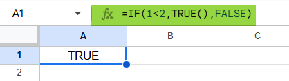
The TRUE formula in Google Sheets is one of the most straightforward. Let us look at a simple example below. With the logical condition, we check if it is true or false. =IF(1<2,TRUE(),FALSE). If true, the function TRUE() returns the logical value TRUE. TRUE in Google Sheets may not be the most powerful formula, but combined with other logical functions like IF and AND, it forms the cornerstone of many complex formulas.
Use this TRUE in Google Sheets Template to follow along with the examples in this article.
Download Excel TemplateKey Takeaways
- The function =TRUE() is a built-in function in Google Sheets that returns the Boolean value TRUE. 2.
- Its syntax is TRUE(), without any arguments. If you enter =TRUE() in any cell, the function will return TRUE. 3.
- TRUE is commonly used with IF statements and logical functions like AND, OR, and NOT to represent conditions that evaluate to true. 4.
- It is extremely helpful to use TRUE in conditional formatting rules to highlight cells based specific conditions. 5.
- In Boolean logic, the value TRUE represents a true condition, while FALSE evaluates to a false condition.
Syntax
As seen below, the syntax of TRUE in Google Sheets is as follows:
=TRUE()
As you can see, there are no arguments. Such Boolean values are fundamentally essential for conditional statements we often use in our calculations. It shows that you can simply use the TRUE function along with logical functions like IF, AND, and OR to get solutions for complex operations without passing any parameters.
Remember, Google Sheets converts the text TRUE to logical TRUE. So, we just key in the word TRUE, and the sheet interprets it as the logical TRUE.
How to Use TRUE Function in Google Sheets?
We can calculate TRUE in Google Sheets in two ways.
- Entering TRUE in Google Sheets manually
- Access from the Google Menu bar
Entering TRUE in Google Sheets Manually
Let us look at how to manually enter the TRUE function to solve certain conditional statements in Google Sheets.
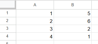
Step 1: First, enter a set of numbers in Google Sheets. We aim to print “TRUE” if the condition holds true and “FALSE” if the condition is not met.
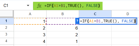
Step 2: Next, apply the formula and select the cell where you want to enter the formula. Here, we select cell C1. Type the following formula IF(A1>B1,TRUE(), FALSE) in the cell.
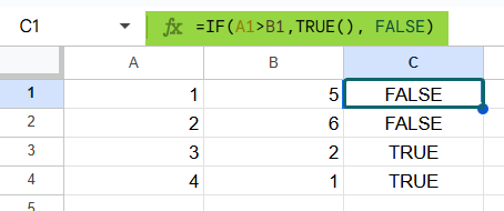
Step 3: Press Enter after closing the braces. Thus, you get the result of TRUE if the condition is true and False otherwise. Drag the formula down to D4 to get the results for all the values.
Access From the Google Menu Bar
Choose any cell and go to the “Insert” tab. Go to the option Function and click on the “Logical” drop-down arrow. From there, choose the TRUE function to insert into your formula.
Examples
The best part about using TRUE is that if you manually type TRUE in a cell, it is recognized as a logical value, not a string.
It becomes very helpful when combined with other functions to perform calculations, set up conditional formatting rules or filter required data. Let us look at how to implement TRUE with some suitable examples.
Example #1
The most basic use of TRUE in Google Sheets is to insert the Boolean value TRUE into a cell. Besides this, we specify a few more conditions and look at how TRUE behaves in each scenario.
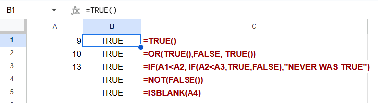
Step 1: Let us enter the following TRUE functions in a sheet. Before that, we also entered a few values in A1, A2, and A3.
=TRUE()
=OR(TRUE(),FALSE, TRUE())
=IF(A1<A2, IF(A2<A3,TRUE,FALSE),”NEVER WAS TRUE”)
=NOT(FALSE())
=ISBLANK(A4)
Step 2: Press Enter as you copy each formula and check the results.
Explanation:
=TRUE(): the formula =TRUE() returns the Boolean value TRUE.
=OR(TRUE(),FALSE, TRUE())
- The OR function checks if any of the arguments given as parameters evaluate to TRUE.
- TRUE() returns TRUE; hence, we get TRUE because of the first argument, irrespective of the other values.
=IF(A1<A2, IF(A2<A3,TRUE,FALSE),”NEVER WAS TRUE”)
The outer IF condition evaluates to TRUE as 9 < 10. Now, the second IF function will be evaluated. Here, 10 < 13. Since this is also TRUE, the formula returns TRUE.
=NOT(FALSE())
Here, the FALSE() returns the Boolean value FALSE, and the NOT function reverses the logical value. Hence, it returns TRUE.
=ISBLANK(A4)
This formula easily returns TRUE as cell A4 is blank.
Example #2 – Using TRUE in Conditional Formatting
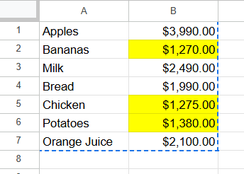
You can also use the TRUE function in conditional formatting where its use truly shines! You can use it in different ways. For example, you can use =A5=TRUE to apply conditional formatting to all cells whose value is true. Let us consider a scenario in our example. We have the sales details of a store and want to flag all sales below a particular value so that they can be boosted. By using the TRUE function, you can easily identify these entries. Let us see how to use the formula in such a scenario.
Step 1: Enter the sales details of different items in a sheet.

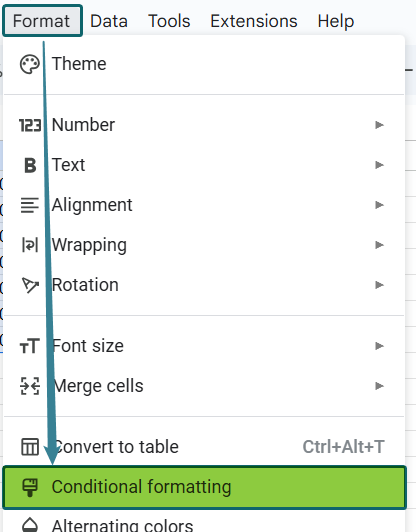
Step 2: Let us apply a new conditional formatting rule. Go to Format -> Conditional Formatting.
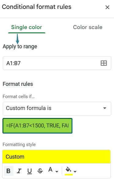
Step 3: You get the “Conditional Format rules” window on the left side of the sheet. Click on “Add another rule” and select the required range where you want to apply the formatting under “Apply to Range.”

Step 4: Choose “Custom formula is” under the “Format cells if..” option. With this, you can apply Google Sheets conditional formatting custom formula.
=IF(A1:B7<1500, TRUE, FALSE). This function will tag each sale below $1,500 as TRUE, simplifying your task of identifying areas of improvement.
Now, choose a custom color under the formatting style.
Step 5: Press Done. You can see the cells highlighted for the cell values in Column B less than $1500.
Thus, the function, when it outputs the logical value TRUE, is used for conditional formatting, among its various other uses.
Example #3 – Using TRUE with AND Function
In Google Sheets, the AND function can be used along with TRUE to create complex conditions. The AND function works as follows: it returns TRUE if all arguments are logically true and FALSE if any arguments are false. Let us use AND as well as TRUE to solve an issue. A table is created where some students in Maths, English, and Science marks are added.
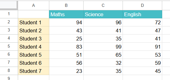
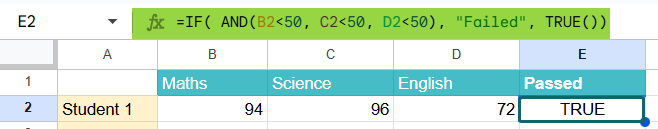
Step 1: We use the AND function to check whether the student failed in every subject. Then, they are assigned the term “Failed.” Enter the following formula in cell E2.
=IF( AND(B4<50, C4<50, D4<50), “Failed”, TRUE())

Step 2: Press Enter. As the first student has grades in all subjects above 50, the AND function evaluates to FALSE. So, we just print TRUE to understand the workings of the function TRUE.
Step 3: Drag the function for all the students and check the result. Whenever a student has grades less than 50 in all three subjects, the AND function evaluates to TRUE, and we get the string “Failed.”

Thus, as you can see, while TRUE is a function, it also represents a logical value. Above, the AND function in Google Sheets evaluates to a logical TRUE while TRUE() also returns the logical TRUE value. We hope these examples have given you a detailed understanding of the TRUE formula in Google Sheets.
Important Things to Note
- Normally, we use the TRUE function as part of the IF function to create a conditional statement. Besides, it can also be used with AND or OR functions to create logical conditions.
- The TRUE function is case-insensitive. Hence, TRUE(), True, and true will all have the same result.
- The TRUE function does not take any input values.
- TRUE in Google Sheets is treated as a numeric value of 1 in formulas. For example, =TRUE + 2 gives you 3 as a result.
Frequently Asked Questions (FAQs)
Below are a few examples of using the TRUE formula in Google Sheets.
1. It can be used to test other formulas. For example, you can test two values and use =IF(B3>C3,TRUE,FALSE) to find whether the value in cell B3 is greater than in cell C3.
2. It is also used for filtering data. It can be used with the FILER function to filter data based on a specified condition. In this case, the formula will return all values where the corresponding value in column B is true.
3. We can use the TRUE formula in conditional formatting to highlight specific cells for evaluation based on specified conditions.
We may get the #VALUE! error when the TRUE function is used with an incorrect syntax or arguments. Remove any argument and check the syntax to resolve this error.
A #REF! error is displayed when the TRUE function references a cell that does not exist.
If the value TRUE is misspelt, you will get the #NAME? Error.
TRUE is often used in logical functions such as AND, OR, and NOT to specify multiply conditions which can evaluate to TRUE or FALSE.
For instance, =OR(TRUE, FALSE) will return TRUE because one of the conditions is TRUE while =AND(TRUE, FALSE) will return FALSE because both the conditions must be TRUE for the AND function to return TRUE.
Use this TRUE in Google Sheets Template to follow along with the examples in this article.
Download Excel Template