
What Is Waterfall Chart In Google Sheets?
Waterfall chart in Google sheets is an inbuilt chart type used to analyze the data visually. In other words, it is used to find and see the sequential financial changes in the given data. Therefore, data such as revenue, expenses, sales performance can be analyzed visually in Google sheets. It is used to show the value changes with a series of positive and negative data in the spreadsheets.
For example, consider the below table showing name and projects in columns A and B, respectively.
Use this Waterfall Chart In Google Sheets Template to follow along with the examples in this article.
Download Excel Template
Now, let us learn how to use Waterfall chart. To begin with, we need to select the cell range A1:B6 and click on Insert. Select Chart and choose Waterfall chart in the chart drop-down option. We will be able to see the waterfall chart, as shown in the below image.

In this article, let us learn how to create waterfall chart in Google sheets with the help of detailed examples.
Key Takeaways
- Waterfall chart in Google sheets is used to represent data visually.
- It is an inbuilt chart in Google sheets and Excel.
- To create waterfall chart in Google sheets, we need to simply select the cell range we want to include in the chart and click on Insert tab.
- Next, select the Chart option and search for waterfall chart in Google sheets under the chart type drop-down in Chart Editor window.
- This chart is mostly used in financial analysis and is used to represent the sequential financial changes in the given data.
- Likewise, we can represent the changes in revenue, expenses, and sales performance in Google sheets.
- We can create sequential or stacked waterfall charts in Google sheets.
How To Create A Waterfall Chart In Google Sheets?
Let us learn how to create a waterfall chart with the help of the following steps.
The steps are:
Step 1: To begin with, insert the data in the spreadsheet.
Step 2: Next, select the cell range and click on Insert. Next, select Chart and choose Waterfall chart in the chart drop-down option.
Step 3: We will be able to see the Chart Editor window at the right-end of the screen.
Now, choose Waterfall chart in the chart type option.
We will be able to see the result in the spreadsheets in Google Sheets.
Likewise, we will be able to create waterfall chart for the given data and analyze the data efficiently.
Examples
Now, let us understand how to create waterfall chart with detailed examples.
Example #1 – Analyze Sales Performance By Breaking Down Changes In Sales Figures Quarter By Quarter
For example, consider the below table showing sales of various electronic products in a year, categorized in quarters (Q1,Q2,Q3 and Q4) in columns A, B, C, D and E, respectively.

Now, let us learn how to create waterfall chart in Google sheets with the following detailed steps.
The steps are:
Step 1: To begin with, insert the data in the spreadsheet. In this example, the data is available in the spreadsheet A1:E5.
Step 2: Next, select the cell range A1:E5 and click on Insert. Next, select Chart in the list of options.

Step 3: We will be able to see the Chart Editor window at the right-end of the screen.

Then, choose Waterfall chart in the chart drop-down option.
We will be able to see the result in the spreadsheets in Google Sheets, as shown in the below image.

This chart is sequential type waterfall chart in Google sheets.
To create waterfall chart in Google sheets with stacked Stacking type, simply double click on the chart. The Chart Editor window appears. Here, click on the Stacking drop-down option and click on Stacked.
We will be able to see the waterfall chart in Google sheets with stacked type as shown in the below image.

Likewise, we will be able to create waterfall chart in Google sheets to analyze sales performance by breaking down changes in sales figures quarter by quarter.
Example #2 – Track Changes In Expenses Such As Operational Costs, Overhead Expenses, And Salaries
For example, consider the below table showing operational cost, overhead expenses and salaries categorized in regions in columns A, B, C, and D, respectively.

Now, let us learn how to create waterfall chart in Google sheets with the following detailed steps.
The steps are:
Step 1: To begin with, insert the data in the spreadsheet. In this example, the data is available in the spreadsheet A1:D5.
Step 2: Next, select the cell range A1:D5 and click on Insert. Next, select Chart in the list of options.

Step 3: We will be able to see the Chart Editor window at the right-end of the screen.

Then, choose Waterfall chart in the chart drop-down option.
We will be able to see the result in the spreadsheets in Google Sheets, as shown in the below image.

This chart is sequential type waterfall chart in Google sheets.
To create waterfall chart in Google sheets with stacked Stacking type, simply double click on the chart. The Chart Editor window appears. Here, click on the Stacking drop-down option and click on Stacked.
We will be able to see the waterfall chart in Google sheets with stacked type as shown in the below image.

Likewise, we will be able to create waterfall chart to track changes in expenses such as operational costs, overhead expenses, and salaries.
Example #3 – Analyze Changes In Customer Retention Rates By Tracking The Number Of Customers Gained(Acquired) And Lost (Churned) Over A Period
For example, consider the below table showing customer retention rates along with newly acquired and lost customers in columns A, B, and C, respectively.

Now, let us learn how to create waterfall chart with the following detailed steps.
The steps are:
Step 1: To begin with, insert the data in the spreadsheet. In this example, the data is available in the spreadsheet A1:C5.
Step 2: Next, select the cell range A1:C5 and click on Insert. Next, select Chart in the list of options.

Step 3: We will be able to see the Chart Editor window at the right-end of the screen.

Then, choose Waterfall chart in the chart drop-down option.
We will be able to see the result in the spreadsheets.

This chart is sequential type waterfall chart.
To create waterfall chart with stacked Stacking type, simply double click on the chart. The Chart Editor window appears. Here, click on the Stacking drop-down option and click on Stacked.
We will be able to see the waterfall chart with stacked type as shown in the below image.

Likewise, we will be able to create waterfall chart to analyze changes in customer retention rates by tracking the number of customers gained (acquired) and lost (churned) over a period.
Important Things To Note
- Waterfall chart is a default function.
- It is used to analyze the data efficiently.
- Remember, we can create waterfall charts to analyze financial data.
- To change the stacking type, we can easily select the Chart Editor Window and click on the Stacking drop-down option.
- The sequential chart type shows each data in a waterfall chart type method whereas, the stacked chart type shows the data stacked on top of each other.
Frequently Asked Questions (FAQs)
For example, consider the sample list and data in columns A and B, respectively.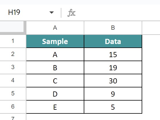
Let us learn how to create a waterfall chart in Google sheets with the help of the following steps.
The steps are:
Step 1: To begin with, insert the data in the spreadsheet. In this example, the data is available in the cell range A1:B6.
Step 2: Next, select the cell range and click on Insert. Next, select Chart and choose Waterfall chart in the chart drop-down option.
Step 3: We will be able to see the Chart Editor window at the right-end of the screen.
Now, choose Waterfall chart in the chart type option.
We will be able to see the result in the spreadsheets, as shown in the below image.
Likewise, we will be able to create waterfall chart for the given data and analyze the data efficiently.
In Google sheets, we will be able to create two types of charts under waterfall chart. We can create sequential or stacked waterfall chart type. We can change the chart type in the Chart Editor window under Stacking option.
Waterfall chart in Google sheets may not work if the data is not available in numeric formats. We need to ensure that the data must be in numeric formats like number, accounting, financial or percentage. The chart will not appear if the data is in Plain text format.
Use this Waterfall Chart In Google Sheets Template to follow along with the examples in this article.
Download Excel Template