What Is Break Links In Excel?
Break links in Excel is an option that severs the connection between cells and worksheets across multiple workbooks. And the process involves breaking a link to the external source file in the active worksheet.
Users can break links in a spreadsheet to improve its performance and ensure data security or when the source files specified in the external links get deleted.
For example, the image below shows three workbooks.
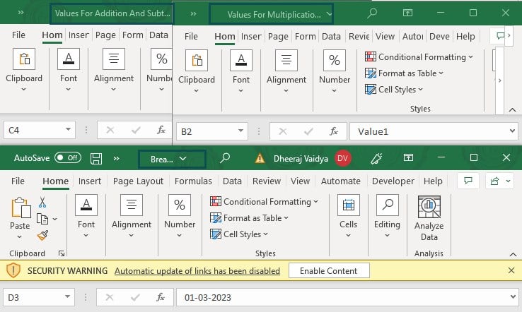
The first two workbooks contain values for addition, subtraction, multiplication and division operations in the target cells B2:B5 in the third workbook. And we use external links to refer to the first two workbooks’ values in the third workbook.
If the requirement is to find and break links in Excel sheet Arithmetic Operations in the third workbook.
Then, as the third workbook has only one worksheet with four cells containing external links to two workbooks, we do not have to search the entire workbook for all the external links.
And, considering the break links in Excel meaning explained above, we can use the Break Link option in the Edit Links function in the Data tab.
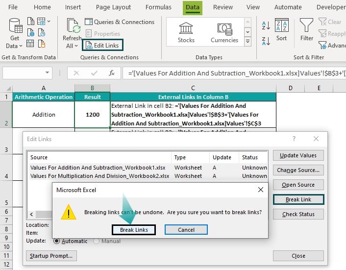

We must choose the Edit Links function in the Data tab to open the Edit Links window. The window shows the two source workbooks to which the active worksheet has external links.
Next, we click inside the section showing the sources and select the two concerned sources in the Edit Links window. And then click the Break Link button on the right, which will show a warning message stating that breaking external links is irreversible.
We can click Break Links in the warning message box to proceed.
Finally, we will see arithmetic operation results as values in the target cells, as shown in the Formula Bar, with the external links in the Edit Links window removed.
Table of contents
Key Takeaways
- Break links in Excel is an option that helps break or sever links in a workbook to external sources.
- Users can break external links in Excel to ensure the program does not slow down and to uphold data security. Also, it is useful when the source files get deleted, and users must break the corresponding external links.
- We can use the Copy and Paste Special as Values option or the Break Link option in the Edit Links function in the Data tab to break external links in Excel.
How To Break External Links In Excel?
We can break external links in Excel using the following two methods:
- Using the Copy and Paste as Values Option
- Using the Edit Links Option
Method #1 – Using The Copy And Paste As Values Option
- Click the first target cell, press Ctrl, and select all the other target cells where we need to break external links to source data in the active worksheet.
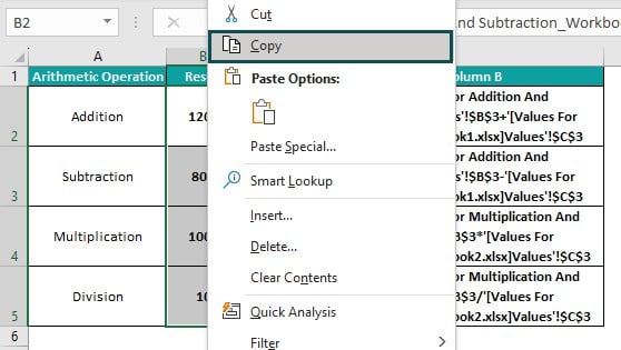
- Right-click on a chosen cell to select Copy from the context menu to copy the cells. Otherwise, press Ctrl + C.
- Right-click on a chosen cell to select Excel Paste Special option – Values from the contextual menu to paste the cells’ data as values.
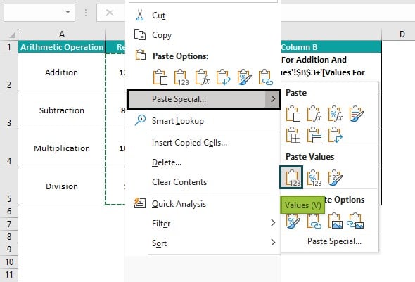
Otherwise, select Paste Special – Paste Special in the context menu or press Alt + E + S to open the Paste Special window. And then, press V to choose the Values option and OK to complete the action.

The above steps will show the values instead of the external links in the target cells.
Method #2 – Using The Edit Links Option
- Select the Data tab – click the Edit Links option to open the Edit Links window.

Please note the Edit Links option will be enabled in the Data tab when the active workbook contains external links. Otherwise, the option will be greyed out, and we cannot break links in Excel using this method.
- Select the first external source to break the corresponding link, press Ctrl, choose the remaining external sources, and press Break Link in the Edit Links window.
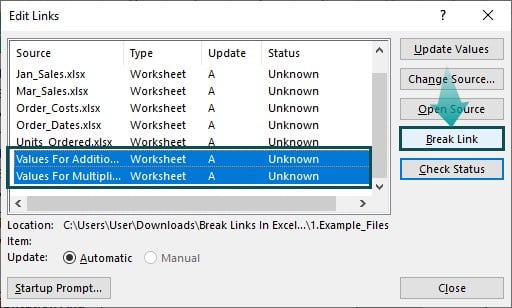
- Excel will show a warning message stating that breaking links will irreversibly change formulas and external references to their current values. Also, it suggests we save the file version in another name. And it asks us whether we are sure to break the chosen links. Click Break Links to proceed.

- We will no longer see the links to the chosen external sources we broke in steps 2 and 3 in the target cells. Instead, the Formula Bar will show the value in the specific target cells.
Further, we can use the break links in Excel shortcut. And for that, press Alt + A + K or Alt + E + K to open the Edit Links window and access the Break Link option. And then, the rest of the process remains the same as explained previously.
Examples
Let us see the examples for understanding the break links in Excel meaning and the two methods explained in the previous section.
Method #1 – Copy And Paste As Values
Consider we have four workbooks. The first three contain the three branch offices’ Jan, Feb, and Mar months sales reports. And the fourth one contains the consolidated sales report based on the first three files.
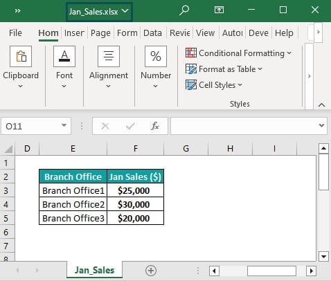


Thus, the fourth file contains external links. And the requirement is to find and break links in Excel file. Then, the steps are as follows:
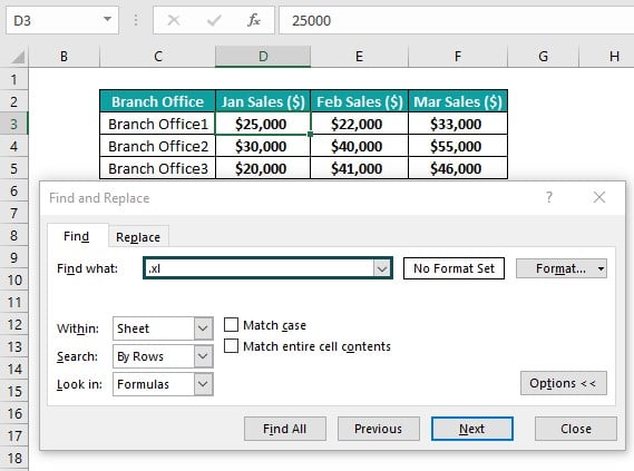
Step 1: Press Ctrl + F to open the Find tab from the Find and Replace dialog box.

As external links will contain Excel extensions for files, enter “.xl” in the Find what field. And click Options.

Ensure the settings search the specified term within the current sheet by rows and formulas.

And then, press Find All in the Find and Replace window.
Excel will list all the cells in the active workbook containing the file extension with the term “.xl”.
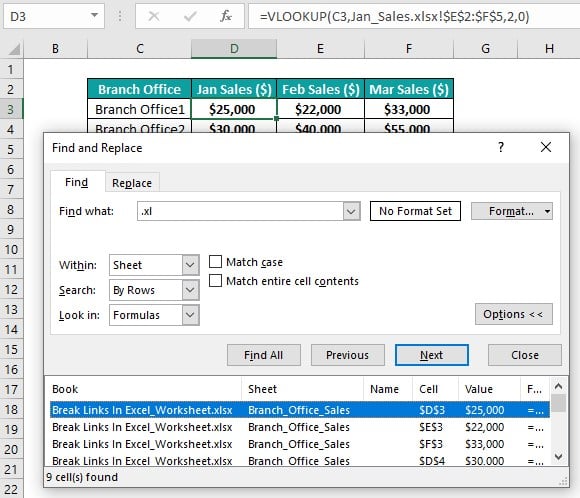
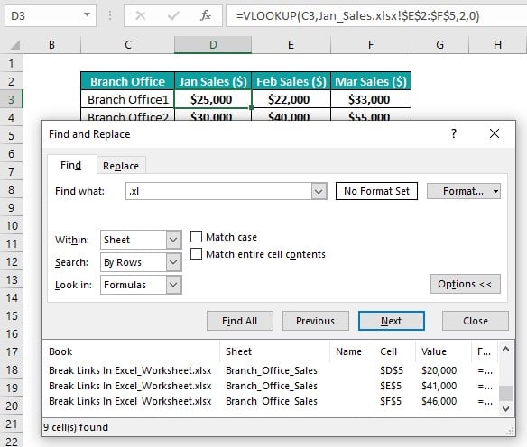
Next, check if the listed cells contain the external links since Excel would also list those cells containing the phrase “.xl” as a part of file names and not external links.
And once confirmed, proceed with step 2.
Step 2: As the first source appears selected in the list, press Ctrl + A to choose all the cells containing the external links.

Step 3: The required cells appear selected. So, right-click on a chosen cell to select Copy from the context menu.


And then, right-click on a chosen cell again to select Paste Special – Values.

Alternatively, select Paste Special – Paste Special in the context menu or press Alt + E + S to open the Paste Special window. And then press V to choose Values to paste the copied data as values.

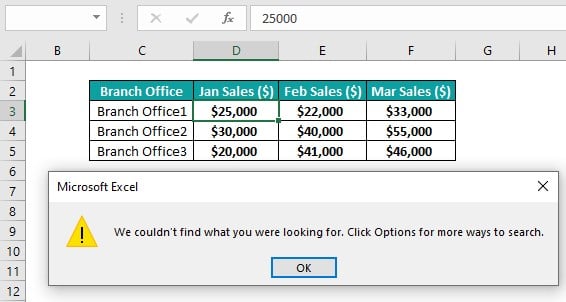
Click OK to view the external links replaced with values in the chosen cells. And if we press Ctrl + F to open the Find tab from the Find and Replace window and search for “.xl”.
Then, Excel will show the message that it could not find the searched phrase.
Likewise, we can copy the cells containing external links and paste them as values in new cells using the Paste Special as Values option.
However, if the external links are hidden, such as those in charts, we cannot break links in Excel. The reason is that the Find option will not list the cells containing hidden links.
Method #2 – Edit Links Option
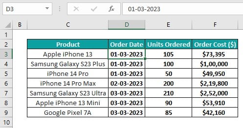
We have four workbooks. While the first three contain the order dates, units ordered, and per unit costs data, the fourth workbook contains the listed products’ order data based on the three files’ data.
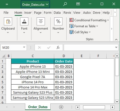


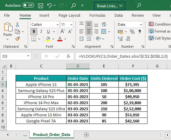
Thus, the fourth workbook contains external links to the source data in the first three files.
And the requirement is to break the links in the active worksheet in the fourth workbook. Then, the steps to use the Edit Links option to break the required links are as follows:
Step 1: Click on Data – Edit Links.
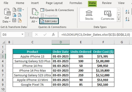
The Edit Links window will open, listing all the sources to which all the worksheets in the active workbook have external links.
Alternatively, use Alt + A + K or Alt + E + K as the break links in Excel shortcut to open the Edit Links window and access the Break Link option.
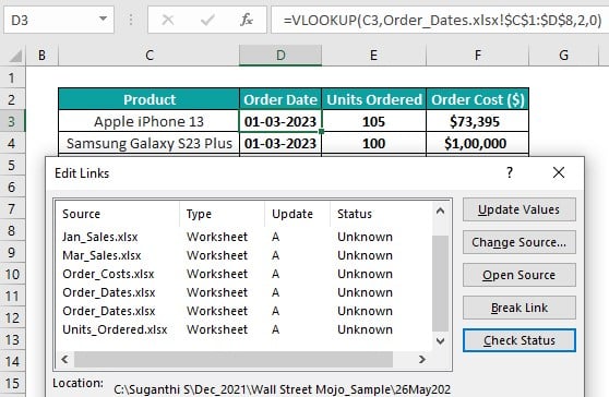
Next, in the fourth workbook, we must break the external links to the source workbooks, Order_Costs, Order_Dates, and Units_Ordered.
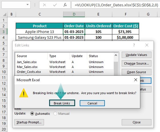
Step 2: Select the Order_Costs.xlsx source in the list. And then, press Ctrl, and select the last two entries in the list to choose the remaining corresponding sources.

Next, click Break Link.
Excel will show the warning message whether to proceed with the breaking links process. Click Break Links to confirm the same.
While the sources in the external links we broke get removed from the list in the Edit Links window, the cells previously containing external links show values in the Formula Bar.
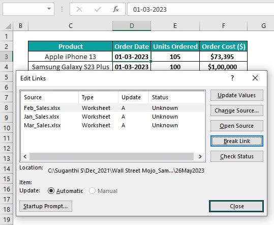
Click Close to close the Edit Links window.
Please note that if any objects, such as text boxes or charts, contain external links, the links will be hidden. But the Edit Links window will list their sources, and we can break the required links as explained above.
Important Things To Note
- Once we break links in Excel, we cannot undo the action. Thus, it is best to save a version of the file with the external links, in another name, before breaking the links.
- Use “.xl” in the Find and Replace window to search for cells containing external links.
- Use the Break Link option in the Edit Links window to break links when the specific workbook contains external hidden or ghost links.

Frequently Asked Questions (FAQs)
We can break links in Excel when source not found in the following ways:
• Delete the named ranges in the workbook to break the external links.
• Check the objects, such as text boxes, for external links to break them.
• Zip the Excel workbook.
• Change the active file extension.
You can break a ghost link in Excel using the Break Link option in the Edit Links window.
For example, the workbook below contains a Line plot.
However, the Edit Links option in the Data tab appears enabled, indicating the workbook contains external links.
And clicking the Edit Links option in the Data tab opens the Edit Links window, showing one source to which the current workbook has an external link.
Thus, here is how to break the ghost links.
1: The workbook contains only one sheet with a Line plot. So, we will click the chart area to enable the Design tab and click the Select Data option to check if the chart data range contains the external link.
And the Chart data range field does show the data range with the external link we considered a ghost link.
Click OK to close the link.
2: Click the Edit Links option in the Data tab to open the Edit Links window.
And then, click the source, to which the current workbook has an external link, to select it and click the Break Link option.
Next, click Break Links in the warning message box to proceed with breaking the link.

Finally, click Close to close the window.
Please note that the external source still appears in the Edit Links window.
However, if we check the chart data range in the Select Data Source window, the field will be empty, indicating the external link or the ghost link is broken.
In the above scenario, deleting the chart data range in the Select Data Source window will do the job since we found out where the external ghost link got used.
However, when we cannot find where the external ghost link is used in a workbook, we can use the Break Link option in the Edit Links window to break it.
You can’t break all links in Excel, perhaps because some worksheets containing external links are password-protected in the active workbook.
Download Template
This article must be helpful to understand the Break Links In Excel, with its formula and examples. You can download the template here to use it instantly.
Recommended Articles
This has been a guide to What Is Break Links In Excel. Here we learn how to break external links in Excel using top 2 methods along with examples and points to remember. You may learn more from the following articles –

Leave a Reply