BYROW in Google Sheets

What Is BYROW in Google Sheets?

The BYROW function in Google Sheets allows you to apply a LAMBDA function to each row of a specified array or range. It returns the results as a new column array, with each value in the new column representing the result of the LAMBDA function applied to the corresponding row in the original array.

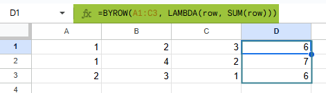
BYROW is designed to perform calculations or operations on a row-by-row basis within a given dataset. It is integrated with the LAMBDA function, which allows you to define a custom function to be applied to each row. The function outputs a new column array. As an example, to find the sum of each row in the range A1:C3, we use the following formula:

=BYROW(A1:C3, LAMBDA(row, SUM(row)))

In this example, BYROW iterates through each row in A1:C3. For every single row, the LAMBDA function calculates the SUM of that row, and the results are returned as a column array.

BYROW in Google Sheets applies a formula to each row in a specified array or range, returning a single result per row.
The function is useful when you need row-level calculations (e.g., sum of values etc.
The syntax of the BYROW function is as follows: =BYROW(array, LAMBDA(row, formula))
1. array → the range to process row by row
2. LAMBDA(row, formula) → defines the calculation for each row
BYROW outputs results vertically down a single column, with one value corresponding to each row in the input array.
For element-wise operations across a range, use ARRAYFORMULA; for column-wise aggregation, use BYCOL.

Syntax

The BYROW in Google Sheets formula is as follows:

=BYROW(array_or_range, lambda)

Arguments:

array_or_range: The range of cells or array to which the LAMBDA function will be applied.
lambda: The LAMBDA function that defines the operation to be performed in each row. The LAMBDA should take a single argument, which represents the current row being processed.

How To Use BYROW Function in Google Sheets?

The BYROW function is used to apply a formula or calculation across each row of a given range. It works with the LAMBDA function to process rows individually and return the results in a column.

It is useful in scenarios where you want to quickly calculate something like row sums, averages, or maximum values without writing formulas separately for each row.

There are two main ways to enter the BYROW function in Google Sheets:

Enter BYROW manually
From the Google Sheets menu

Enter BYROW Manually

Let us look at the manual method to enter the BYROW function. To illustrate this, we will calculate the product of each row in a dataset with the following details:

We have a small table of numbers. We will calculate the product of each row.

Step 1: Open Google Sheets and in a new spreadsheet, enter the required details in cells A1:C3.

Step 2: Enter the BYROW formula in an empty column (say D1). Start with an = sign, followed by the function name and open braces. Enter the arguments in the order specified in the syntax.

=BYROW(A1:C3, LAMBDA(r, PRODUCT(r)))

Step 3: Press Enter. The cells in column D will display the product using PRODUCT of each row:

First row → 30

Second row → 64

Third row → 14

Entering BYROW Through the Menu Bar

Go to the Insert tab.
Choose Function → Array.
From the list, select BYROW.
Fill the arguments in with the proper values (e.g., A1:C3 for the array, and LAMBDA(r, PRODUCT(r)) for the lambda).
Press Enter to get the result.

Examples

Now that we have some idea on how BYROWS works, let us look at some practical scenarios where it can be used with the help of some interesting examples.

Example #1

The BYROW function is not only limited to numbers, it can also process text data. In this example, we will use BYROW along with the TEXTJOIN function to automatically generate full names from first and last name columns. Since it does the processing row by row, we will get the result for the entire range without using ARRAYFORMULA.

Step 1: Set up your range by entering all the details in a new sheet. In the first column, we enter a list of first names, and in the second column, their last names.

In a new spreadsheet, enter the following employee names.

BYROW Function in Google Sheets Example 1

Step 2: Enter the formula

In an empty column (for example, cell C2), enter the BYROW formula:

=BYROW(A2:B5, LAMBDA(r, TEXTJOIN(” “, TRUE, r)))

Here:

A2:B5 → The range with first and last names.

LAMBDA(r, TEXTJOIN(” “, TRUE, r)) → Joins the values in each row with a space.

BYROW Function in Google Sheets Example 1-1

Step 3: Press Enter. The results will appear in column C as full names.

BYROW Function in Google Sheets Example 1-2

This approach helps combine text values row by row automatically, without the need of separate CONCAT formulas.

It’s especially useful in areas such as HR and marketing where you need to create clean full names.

Example #2 – Using BYROW to grade student assignments

Let us use the BYROW function to calculate the average score of students across multiple assignments. For instance, say you have scores of 4 students across 3 assignments, and you want to calculate each student’s average automatically using BYROW.

Step 1: Set up your dataset with the following details in an empty spreadsheet.

BYROW Function in Google Sheets Example 2

Step 2: Enter the following formula in an empty column, say E.

=BYROW(B2:D5, LAMBDA(r, AVERAGE(r)))

Here:

B2:D5 → The scores of students.
LAMBDA(r, AVERAGE(r)) → Tells BYROW to calculate the average of each row.

BYROW Function in Google Sheets Example 2-1

Step 3: Press Enter. The formula will return the average score for each student in column E.

BYROW Function in Google Sheets Example 2-2

The BYROW function helps automate grading by calculating averages row by row, saving time and reducing manual errors.

It is especially useful when dealing with classes and multiple assignments.

Example #3

The BYROW function can be used to automatically calculate total monthly sales when you have multiple representatives or product lines. Instead of writing separate formulas for each row, BYROW processes each row at once.

Step 1: Set up your dataset and enter the sales data for three sales representatives over three months:

BYROW Function in Google Sheets Example 3

Here:

Rep 1, Rep 2, Rep 3 columns show the sales amounts for each representative. It is shown for the month of January, February, and March
Rows → Each row represents a month (Jan, Feb, Mar).

Step 2: In column E, enter the BYROW formula as shown below.

=BYROW(B2:D4, LAMBDA(r, SUM(r)))

Here:

B2:D4 → The range of sales data.
LAMBDA(r, SUM(r)) → For each row (r), BYROW calculates the SUM of sales.

BYROW Function in Google Sheets Example 3-1

Step 3: Press Enter. The results will be displayed in column E as the total sales for each month.

This method allows you to quickly see total monthly sales without manually writing SUM formulas for each row. It’s efficient and scalable for larger sales data.

BYROW Function in Google Sheets Example 3-2

Important Things to Note

The passed LAMBDA accepts only one name argument, otherwise we get the #N/A error. This argument indicates a row in the input array.
Every row should be grouped to a single value. Array results for grouped values aren’t supported.
We can pass a named function to the LAMBDA parameter, which behaves like a LAMBDA in this case.
LAMBDA should have exactly one argument placeholder.

Frequently Asked Questions (FAQs)

When should we use BYROW and when ARRAYFORMULA?

Use BYROW when you want to calculate row-wise sum, averages, max values. When you want to run a function on each row as a unit and return a single result per row, you can use BYROW.

You can use ARRAYFORMULA to apply a formula down a column like math operations, string concatenations etc. In other words, when you want to apply a formula to every row or column without writing it multiple times, you use ARRAFORMULA.

How to use the BYROW function with conditional functions like IF?

At times, we may apply logic based on certain conditions. For instance, we flag the marks secured by students below a certain value.
You enter all the details in a Google Sheet. Enter the BYROW function with the If condition:

=BYROW(D2:D4, LAMBDA(total, IF(marks < 40, “Fail”, “Pass”)))

This will flag the scores below 40 as “Fail” and others as “Pass.”
Thus, BYROW is versatile and can handle different types of data and logic and can be combined successfully with other functions

What are some common errors we get when using BYROW in Google Sheets?

Some of the common errors we get include:

1. #VALUE! Error – We get this error when the LAMBDA function returns a non-numeric value where a number is expected.
2. #REF! Error – We get this error when the range specified doesn’t exist or nor correct. Make sure your range is valid and properly formatted.

Download Template

This article must help understand BYROW Function in Google Sheets with its formulas and examples. You can download the template here to use it instantly.

BYROW Function in Google Sheets Download

BYROW in Google Sheets