
What Is Calculate Age In Google Sheets?
The Calculate Age in Google Sheets helps users to find a person’s age using their date of Birth. We can also find the age in terms of years, months, days, weeks, etc. We do not have a pre-defined Formula to Calculate Age in Google Sheets. So, we can use the TODAY, YEARFRAC or the DATEDIF functions. However, we can use the following Basic Formula to Calculate Age in Google Sheets,
=(Today’s Date-Date of Birth)/365
For example,we can find the age of a person using the Start Date and End Date, as shown below.
Use this Calculate Age In Google Sheets Template to follow along with the examples in this article.
Download Excel Template
Select cell C2, enter the formula =DATEDIF(A2,B2,”Y”) and press “Enter”.

The output is ‘36’, as shown above.
Key Takeaways
- The Calculate Age in Google Sheets helps us find the current age using the date of birth or the number of years using the start and the end dates. We can always use the TODAY() function if we do not have the end date.
- The basic formula to calculate age is (Today’s Date – Date of Birth) / 365. Therefore, Date of Birth is mandatory to calculate the age.
- We can use a few other functions such as the DATEDIF(), YEARFRAC(), and TODAY() for age calculation.
- The two dates compared to Calculate Age must be in the valid format or else the same format, else, we will get an error.
How To Calculate Age In Google Sheets?
Since Google Sheets or MS Excel do not have a pre-defined or built-in formula to Calculate Age, we can build formulas ourselves or create a Age Calculating Template in Google Sheets, using some of the functions such as, DATEDIF(), YEARFRAC(), TODAY(), etc.
In this article, we will use the top four ways to Calculate Age In Google Sheets, namely,
- Basic Google Sheets Formula for Age in Years.
- Calculate Age using the YEARFRAC function.
- Calculate Age using the DATEDIF function.
- Calculate age Using the Array formula.
Examples
We will consider specific examples for the above-mentioned four methods to Calculate Age in Google Sheets.
Example #1 – Basic Google Sheets Formula for Age in Years –
We will use the Basic Formula to Calculate Age in Google Sheets to find the age in years.
In the following table, the data is,
- Column A shows the Name.
- Column B contains the Date of Birth.
- Column C for the Output [Age].

The steps to Calculate Age from Date of Birth using the basic formula are as follows:
Step 1: Select cell C2 and enter the formula =(TODAY()-B2)/365.

Step 2: Press the “Enter” key. The output is ‘29.43013699’, as shown below.

Step 3: As the output is a decimal, not an integer, we will enter the INT formula. Then, the updated formula is=INT((TODAY()-B2)/365) and press “Enter”.
[Note: We can also enter the value of days as 365.25 to be precise instead of 365.]

Now, the exact age is ‘29’, as shown above.
Example #2 – Calculate Age using the YEARFRAC function –
We will first understand the YEARFRAC function.
YEARFRAC function – It calculates the number of whole days between two dates.
The syntax of the YEARFRAC function is,

The arguments of the YEARFRAC function are,
· start_date à It denotes the start date. It is a mandatory argument.
· end_date à It denotes the end date. It is a mandatory argument.
· [day_count_convention] à It denotes the dates fraction. It is an optional argument.
We will use the YEARFRAC function to Calculate Age in Google Sheets.
In the following table, the data is,
- Column A shows the Name.
- Column B contains the Date of Birth.
- Column C for the Output [Age].

The steps to Calculate Age using the YEARFRAC function are as follows:
Step 1: Select cell C2 and enter the =YEARFRAC(B2,TODAY(),1).

[Note: The start_date, i.e., the DOB, is in cell B2. We will take the end_date as today’s date, so use the Today() function and the [day_count_convention] is‘1’].
Step 2: Press the “Enter” key. The output is ’32.83’, as shown in the image below.

Step 3: Since the age is in decimal we can use the INT function like the previous example. Therefore, the new output will be as shown below.

Example #3 – Calculate Age using the DATEDIF function –
We must first understand the DATEDIF function to Calculate Age in Google Sheets.
DATEDIF function – It calculates the number of whole days, full months, or full years between two dates.
The syntax of the DATEDIF function is,

The three mandatory arguments of the DATEDIF function are,
- start_date – It is the start date of the period we want to calculate.
- end_date – It is the end date of the period we want to calculate.
- unit – It is the time unit we want to calculate.
The Unit table is as follows:
| Unit | Name | Explanation |
|---|---|---|
| Y | Years | Several years between the start and end date. |
| M | Months | Number of months between start and end date |
| D | Days | Number of days between start and end date |
| MD | Days excluding year and months | Date difference in days, excluding months and years. |
| YD | Days excluding years | Date difference in days, excluding years. |
| YM | Months excluding days and years | Date difference in months, excluding days and years. |
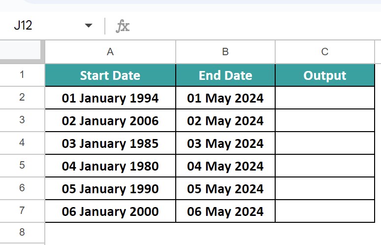
In the following table, the data is,
- Column A shows the Start Date.
- Column B contains the End Date.
- Column C for the Output [Age].

The procedure to Calculate Age in Google Sheets using the DATEDIF function is:
First, select the column C and enter the formulas along with their units as follows,
- In cell C2, enter the formula =DATEDIF(A2,B2,”Y”)
- In cell C3, enter the formula =DATEDIF(A3,B3,”M”)
- In cell C4, enter the formula =DATEDIF(A4,B4,”D”)
- In cell C5, enter the formula =DATEDIF(A5,B5,”MD”)
- In cell C6, enter the formula =DATEDIF(A6,B6,”YD”)
- In cell C7, enter the formula =DATEDIF(A7,B7,”YM”)

After entering the formulas in their respective cells, press the “Enter” key.

We will get the above output shown in Column C. [Note: The results are as per the specified units, w.r.t days, months, years, etc. Column D is for our reference of the applied formulas.]
Example #4 Calculate age Using the Array formula –
In the image below, we have date of birth to calculate the age according to today’s date. We will use the array formula to find the age as per today.

Select cell D2, enter the formula =iferror(datedif(date(C2:C,A2:A,B2:B),date(2024,6,3),”Y”))) and press “Enter”, as shown below.

Now, to execute the formula as an array formula, we must press “Ctrl+Shift+Enter” instead of just the “Enter” key. Then, the formula will become ={ArrayFormula(iferror(datedif(date(C2:C,A2:A,B2:B),date(2024,6,3),”Y”)))}, as shown below.

We can also modify the formula as follows:
={“Age”;ArrayFormula(iferror(datedif(date(C2:C,A2:A,B2:B),date(2024,6,3),”Y”)))},

Here, the output is displayed in cell D3 and the Text Age is displayed in the cell D2.
Important Things To Note
- If we copy the DATEDIF function to another cell in Google Sheets, we will get the #NUM! or #REF! error or just 0 in the cell. Therefore, we should enter the formula manually or drag it in a dataset, since it is not an inbuilt function in Google Sheets.
- We will get the #NUM! error if the end date is less than the start date.
- If Google Sheets does not recognize the valid dates, it returns the “#VALUE!” error.
Frequently Asked Questions (FAQs)
We will Calculate Age in Google Sheets using the DATEDIF and Arithmetic Operations in Completed and Fractional Months.
In the following table, the data is,
The column A shows the Start date.
Column B contains the End Date.
And, column C is for output [Age].
The steps to Calculate Age in Google Sheets, w.r.t months,are as follows:
Step 1: Select cell C2, enter the formula =DATEDIF(A2, B2,“M”) and press “Enter”.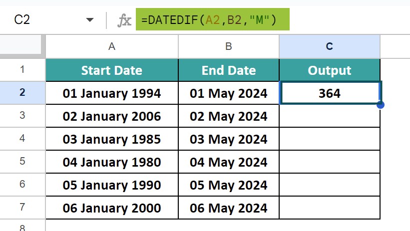
Step 2: Drag the formula from cell C2 to C7 using the fill handle.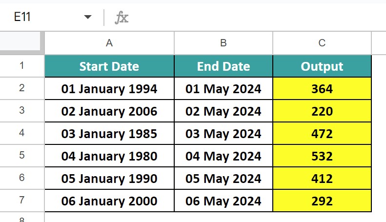
We will get the output as shown above i.e., the number of months between the start and end dates.
We will Calculate Age in Google Sheets using the CONCATENATE and DATEDIF in Years, Months, and Days.
Therefore, in the following table, the data is,
The column A shows the Start date.
Column B contains the End Date.
And, column C is for output [Age].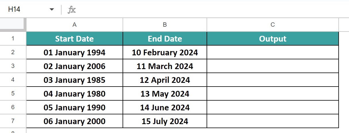
The steps to Calculate Age and display it as a phrase using the CONCATENATE and DATEDIF functions are as follows:
Step 1: Select cell C2, enter the formula =CONCATENATE(DATEDIF(A2,B2,”Y”),”Years “,DATEDIF(A2,B2,”YM”),”Months and “,DATEDIF(A2,B2,”MD”),”Days”) and press “Enter”as shown below.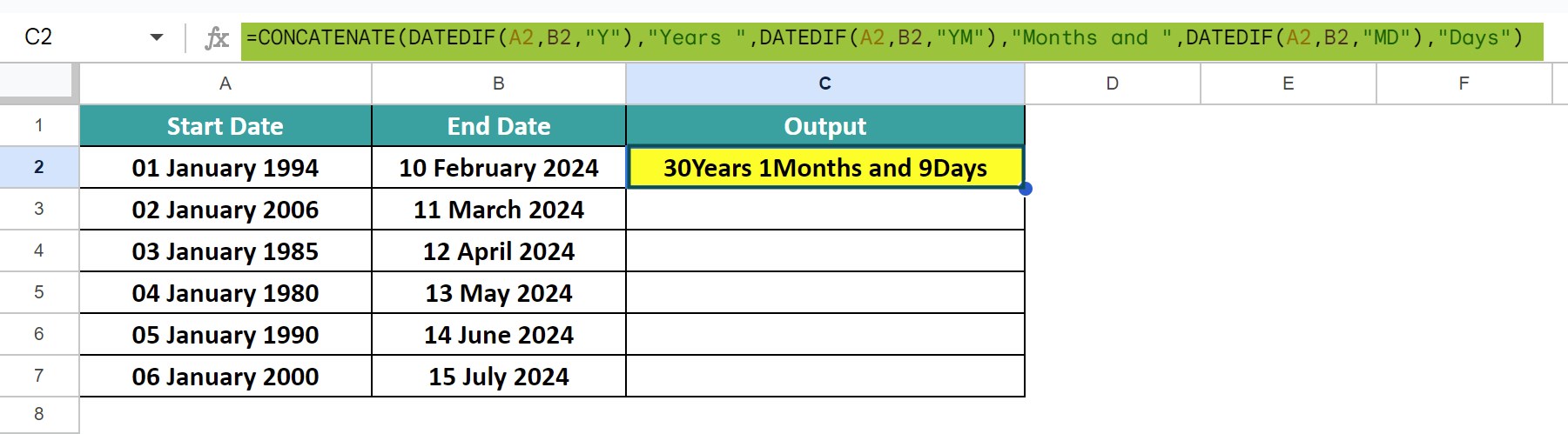
Step 2: Drag the formula from cell C2 to C7 using the fill handle.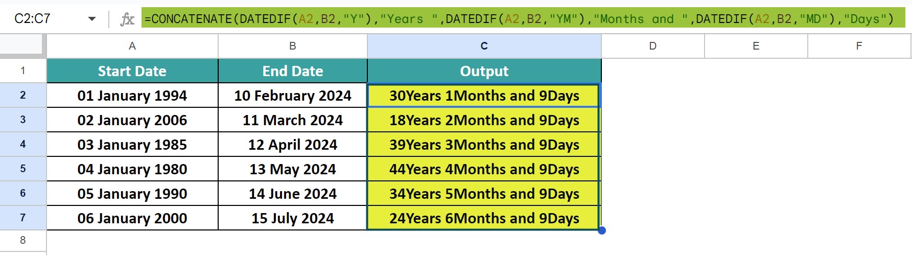
We will get the output shown above. One formula gives the total years, months, and days.
A few reasons the Calculate Age in Google Sheets may not work are,
a. The dates entered are both not in the same valid format.
b. If the values are alpha-numeric, text or blank, then we will not be able to calculate the age.
c. The end date is earlier than the start date.
Use this Calculate Age In Google Sheets Template to follow along with the examples in this article.
Download Excel Template