
What is Compare and Match Columns in Google Sheets?
The Compare and Match Columns in Google Sheets is used to identify the similarities and differences between two or more columns in a Google spreadsheet or across different sheets. We can do this in many ways according to the requirements. This includes finding exact matches, discovering discrepancies, or pinpointing unique values within the data.
We basically use this analysis for data in columns to understand patterns, identify errors, or streamline data management tasks by quickly comparing and highlighting differences, duplicates, or unique values. There are several methods to compare and match columns in Google Sheets such as using formulas with IF, EXACT, and so on. Another way is by highlighting cells based on comparison results with conditional formatting.
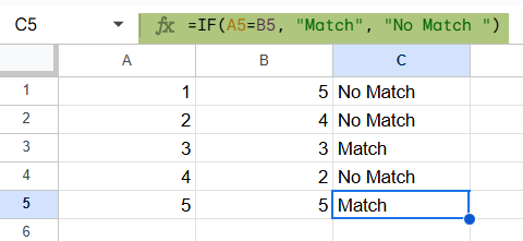
For example, here we use the formula =IF(A2=B2, “Match”, “No Match “)
Use this Compare and Match Columns in Google Sheets Template to follow along with the examples in this article.
Download Excel TemplateKey Takeaways
- Matching and comparing columns in Google Sheets helps identify similarities, differences, or duplicates between data sets in columns. It is important for tasks like inventory checks or list comparisons.
- You can use formulas like IF, EXACT, or COUNTIF to highlight differences when we compare different columns.
- We can also apply conditional formatting to visually distinguish matching or unique entries.
- It can be used for comparing student names, product IDs, or survey responses across sheets.
Top Methods to Compare and Match in Google Sheet
Let us look at the different methods that can be used to compare and match different columns in Google Sheets. Listed below are the most common methods.
#1 – Using The = Operator
We use the = operator for row-by-row comparison of data. This technique in data analysis is a simple yet effective way to compare the values in two columns.
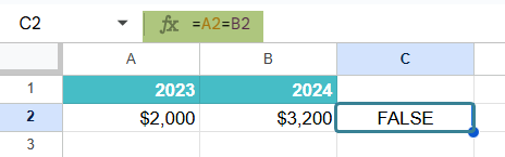
For example, here we identify if the sales figures of a product vary across two years or are consistent using the = operator.
Apply it by inserting ‘=C2=D2‘ in a new column to compare the sales of 2023 and 2024.
#2 – Using IF Function
Another method to compare and match columns is by using the IF function. You can customize your own formula that checks if the values in two columns are equal. The formula is written such that it gives one value if the cells match and a different value if they don’t match.
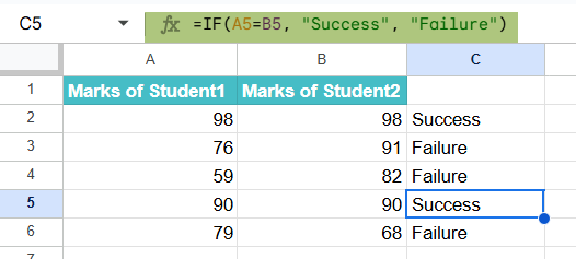
Here, we will display the results of the comparison in Column C.
Enter the following formula:
=IF(A2=B2, “Success”, “Failure”)
#3 – Using The EXACT Function
We can compare columns in Google Sheets using the EXACT function. When we use the EXACT function in Google Sheets in a formula, it returns TRUE if the values are identical and FALSE if they differ. It includes capitalization as well. You can use this to highlight discrepancies.
We enter the details in columns A and B. In Column C, enter the following formula:
=EXACT(A1, B1)
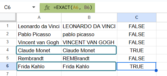
The formula checks if the value in cell A1 is the same as the value in cell B1. The EXACT function is case-sensitive, hence, those cells that contained different cases returned a FALSE for the formula.
Examples
Let us look at some interesting examples of how to match and compare columns in different ways with some interesting examples.
Example #1 – Comparing and Matching Multiple Columns
We have three different columns containing names in a sheet. Let us compare them to find which of the columns has values that match across all of them. We can also single out rows with unique values in each column. This sort of comparison is helpful to verify data.
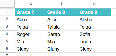
Let us find the names that appear in all three columns.
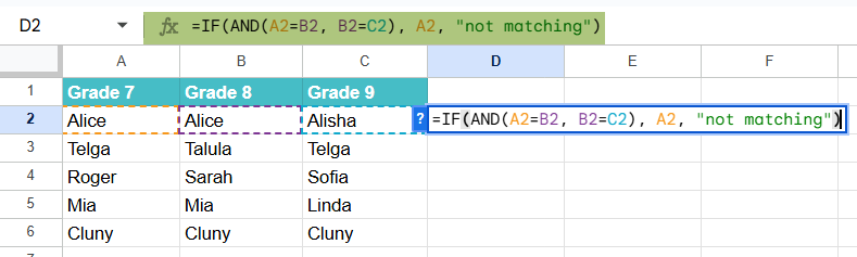
Step 1: Go to cell D2 and type the following formula. We use the IF function and the AND function.
=IF(AND(A2=B2, B2=C2), A2, “not matching”)
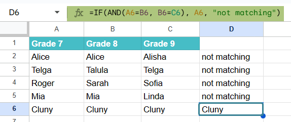
Step 2: Drag the formula up to cell D6 to apply it to all the rows. The formula checks if the name in Column A matches the one in Column B. We then compare it to the name in Column C. If all three match, it returns the name, else it returns “not matching.”.
Example #2 – Case-Sensitive Comparison and Matching
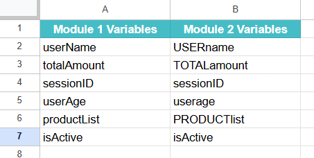
Let us compare two columns where the values look the same but differ in their case. There are many instances where case sensitivity is important and two similar words should not be treated as equal. Google Sheets is not case-sensitive by default and we must apply a formula for the same.
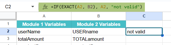
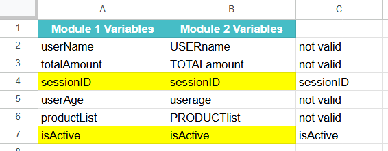
Step 1: We have a Google sheet with some variable names used in two modules of a project in Columns A and B.
Step 2: In cell C2, enter the following function:
=IF(EXACT(A2, B2), A2, “”)
Step 3: Drag the formula down through C7.
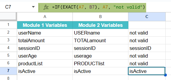
The result will show only the values where both text and case are the same. The EXACT function checks both the text and the case and can be used for strict comparisons.
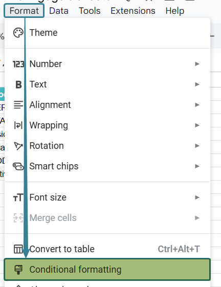
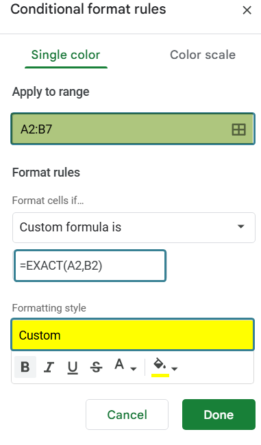
Step 4: We can highlight those rows with an exact match in the case by applying this formula to conditional formatting. Go to Format -> Conditional Formatting.
Step 5: Under Conditional Format rules, go to “Format cells if” and choose “Custom Formula.”
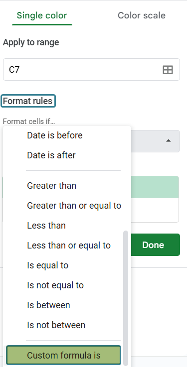
Step 6: Enter the following formula in the box.
=EXACT(A2,B2).
Choose an appropriate color under formatting style. Don’t forget to set the range where you wish to apply this formatting under “Apply to range.” Press Done.
You can observe that all the rows that have the same value including the case have been highlighted.
Example #3 – Comparing and Matching Columns Across Spreadsheets
In this example, we will compare and match columns across different Google sheets. For this, we use formulas such as IF, MATCH, VLOOKUP, or ARRAYFORMULA with conditional formatting. This example shows us how to use VLOOKUP and IF to find matching entries between two different sheets.
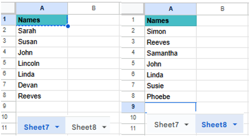
Step 1: Set up the data across two different sheets.
Step 2: In Sheet7, let us use the VLOOKUP in the Google Sheets function to search for values in the other sheet. In cell B2 of Sheet7, use the following formula.
=VLOOKUP(A2, Sheet8!A:A, 1, FALSE)
This will search for the value in A2 in Sheet7 in Sheet8 and if a match is found, it will return the corresponding value from column A of Sheet8.
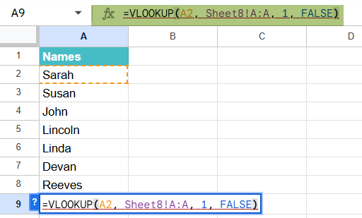
Here, we get #N/A as “Linda” isn’t present in Sheet8.
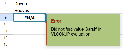
Step 3: We use the IF statement to check if the VLOOKUP returned a value or a #N/A error.
Use the following formula in Sheet7.
=IF(ISERROR(VLOOKUP(A2, Sheet8!A:A, 1, FALSE)), “No Match”, “Match”).
This will display “Match” if a value was found by VLOOKUP and “No Match” if there was no match.
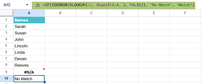
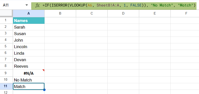
We get “No Match” to replace the #N/A error seen earlier. Now, let us replace A2 with A6. We are searching for Linda which can be found in Sheet8 as well. We enter,
=IF(ISERROR(VLOOKUP(A8, Sheet8!A:A,1, FALSE)), “No Match”, “Match”)
and press Enter. We get a match.
Important Things to Note
If the sheets you wish to compare are in different files, you can use the IMPORTRANGE function.
Another important method we use to find differences or similarities when comparing columns is using conditional formatting.
By default, comparisons of columns in Google Sheets are not case-sensitive. To perform a case-sensitive comparison, we use the EXACT function instead of formulas like A1=B1.
To compare full columns, use formulas like COUNTIF or MATCH. For instance, =IF(COUNTIF(C:C, A2), “Yes”, “No”). It checks if each value in column A exists in column B somewhere.
Frequently Asked Questions (FAQs)
While we try to compare and match columns, we should be aware of some errors that may occur.
They include:
1. Case-Sensitivity: Remember that comparisons in Google Sheets are case-sensitive by default. To ignore case differences, you can use a formula like =UPPER(A2)=UPPER(C2)
2. Mismatched data types: It is important to see that both columns have the same data format. If the columns have different data types, it could lead to inaccurate results.
3. Inaccuracy in formulas: Always check that the formulas used refer to the correct columns and rows, as mistakes may yield unexpected results.
While matching values in columns, one can use the COUNTIF function to check if a value in one column appears in another.
For example, if there are some values in Column A and you wish to find them in Column B, you must use the following formula.
=IF(COUNTIF(B: B, A2)=0, “Only in A”, “”). Here, we get the result “Only in A” if the value in A2 is not found in Column B. We can use it to find unique entries,
To highlight cells that are a mismatch, we use Conditional formatting as follows:
1. Select both columns A and B. For instance, A2:B20).
2. Go to Format > Conditional formatting.
3. Under Custom formula is, enter the following formula: =A2<>B2
4. Pick a color under Formatting style to highlight differences.
It will mark any mismatches between the two columns.
Use this Compare and Match Columns in Google Sheets Template to follow along with the examples in this article.
Download Excel Template