What Is Excel String Concatenation?
Concatenate strings in Excel is an operation that enables one to join two or more text strings into one string. And we can combine cell values, manual data, and strings using the CONCAT(), TEXTJOIN(), and the Ampersand symbol (‘&’).
Users can concatenate strings in Excel during data analysis and while preparing reports in a spreadsheet.
For example, the table below lists US states and their population statistics.
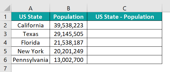
And the requirement is to concatenate the data, given in the two columns, as strings and display the output in column C, with the format as in the column C heading.
Then, we can use the CONCAT()– based concatenate strings in Excel formula in the target cells and obtain the desired output.

In the above example, the concatenate strings in Excel formula is the CONCAT(), with the Excel TEXT function applied inside the CONCAT().
First, the TEXT() returns the column B cell value in the specified format to match the source data format in column B. And then, the CONCAT() combines the column A cell value, the ‘ – ‘ with a space character before and after the hyphen, and the TEXT() output in the corresponding target cells.
Thus, we obtain the concatenated strings in the desired format in the corresponding target cells in column C.
Table of contents
Key Takeaways
- The techniques to concatenate strings in Excelhelp us combine or join multiple text strings, which can be cell values and texts to be entered manually.
- Users can perform Excel string concatenation to make financial and statistical data more understandable and meaningful for other users accessing the data.
- We can concatenate strings in a worksheet using the TEXT functions, CONCAT and TEXTJOIN, and the Ampersand symbol (‘&’).
- We can use the methods to concatenate strings with other Excel inbuilt functions, such as LEFT, RIGHT, and IF, for practical results.
How To Do Excel String Concatenation?
We can concatenate strings in Excel using the following methods:
- Using The Ampersand Symbol (‘&’)
- Using The CONCAT()
- Using The TEXTJOIN()
Method #1 – Using The Ampersand Symbol (‘&’)
The steps to perform Excel string concatenation using the Ampersand symbol (‘&’) are as follows:
- Choose the target cell to show the output.
- Enter the ‘=’ sign, the first cell value or reference to the cell containing the first value, and then the Ampersand symbol (‘&’). Next, enter the remaining cell values or Excel cell references to the values, required texts and manual values, with the ‘&’ symbol entered between each value.
- Press Enter to view the concatenated string in the target cell.
Further, the ‘&’ symbol does not concatenate strings from multiple cells into a single cell with delimiters and separators. Thus, we must provide the separators such as a space character, comma, and full stop in the formula at the positions where they must appear in the final concatenated string.
Method #2 – Using The CONCAT()
The steps to perform Excel string concatenation by applying the CONCAT() are as follows:
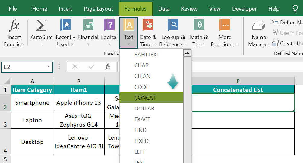
- Select a target cell and choose the Formulas tab → the Text drop-down → choose the CONCAT function.
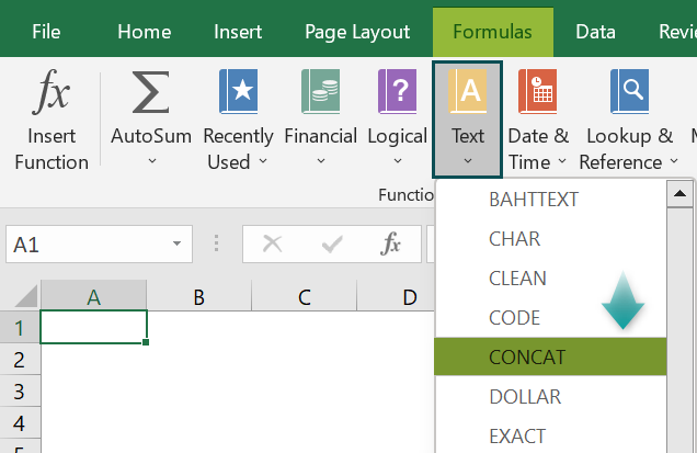
- The Function Arguments window will open, where we must update the mandatory Text1 field, followed by the required number of optional fields Text2, Text3,….. And the inputs can be values or cell references to values.

The CONCAT() can accept up to 255 arguments as input. And if the resulting concatenated string contains over 32767 characters, the function returns the #VALUE! error.
- Click OK in the Function Arguments window to view the CONCAT() output in the target cell.
Alternatively, we can directly enter the CONCAT() in the target cell using the following steps:
- Select a target cell to display the output.
- Type =CONCAT( in the target cell. [ Alternatively, enter =C or =CON and double-click the CONCAT function from the Excel suggestions.]
- Provide the arguments as cell values or references to the values and close the brackets.
- Press Enter to execute the function and view the required concatenated string.
Ensure the supplied arguments are valid and without syntax errors in both methods. Otherwise, we may face a scenario of the concatenate strings in Excel not working.
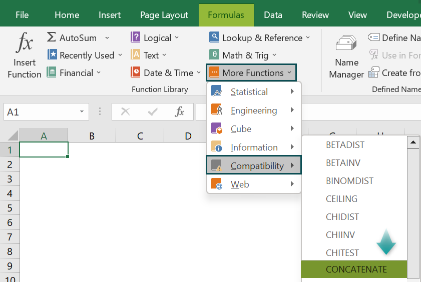
Furthermore, the Excel CONCATENATE function is the older version of the CONCAT(). And while it has the same functionality as the CONCAT(), it is available as a Compatibility function under the More Functions group in Excel.
Method #3 – Using The TEXTJOIN()
The steps to perform Excel string concatenation by applying the TEXTJOIN() are as follows:
- Choose a target cell and select the Formulas tab → the Text drop-down → choose the TEXTJOIN function.
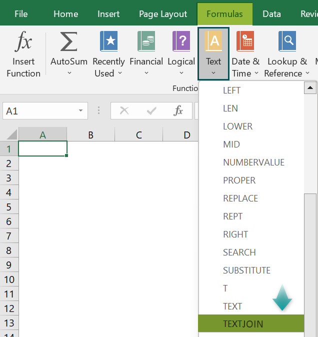
- The Function Arguments window will open, where we must update the mandatory Delimiter, Ignore_empty, and Text1 fields. And once we click in the Text1 field, the optionalfields Text2, Text3,…. Appear one by one, which we can update according to the requirement. And the inputs can be values or cell references to values.
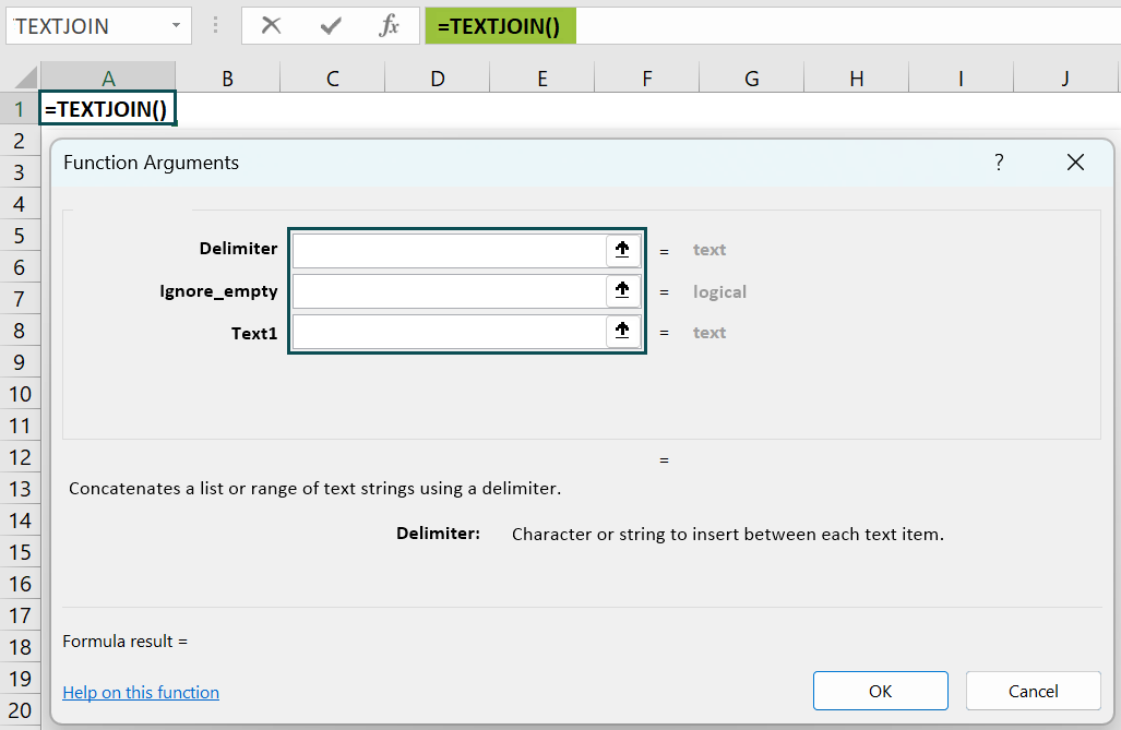
The TEXTJOIN() can accept three mandatory and up to 252 text arguments as input. And if the resulting concatenated string contains more than 32767 characters, the function returns the #VALUE! error in Excel.
- Click OK in the Function Arguments window to obtain the TEXTJOIN() output in the target cell.
Alternatively, we can directly enter the TEXTJOIN() in the target cell using the following steps:
- Choose a target cell to display the output.
- Type =TEXTJOIN( in the target cell. [ Alternatively, enter =T or =TEX and double-click the TEXTJOIN function from the Excel suggestions.]
- Provide the arguments as cell values or references to the values and close the brackets.
- Press Enter to execute the function and view the required concatenated string.
Ensure the provided arguments are valid and do not have syntax errors in both methods. Otherwise, we may face a scenario of the concatenate strings in Excel not working.
Furthermore, the advantage of using the TEXTJOIN() is that we can specify the delimiter we wish to insert between each string value as an argument value.
Also, all the above Excel string concatenation methods are case-sensitive.
Examples
Check out the following concatenate strings in Excel examples to use the option effectively.
Example #1 – Basic Example Of Concatenating Values Into One
We can concatenate strings in Excel with a separator, ‘,’.
For example, the table below shows three item categories, with three items in each category.

And the requirement is to create a concatenated list of all items for each category and display the output in column E.
Then, we can concatenate strings in Excel with a separator, ‘,’, using the CONCAT() and TEXTJOIN(). And the steps are as follows:
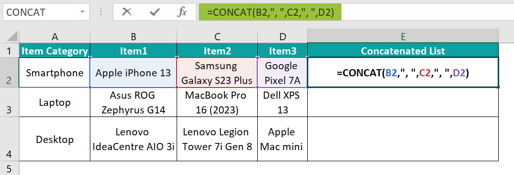
- Step 1: Choose cell E2 and enter the CONCAT().
=CONCAT(B2,”, “,C2,”, “,D2)
- Step 2: Press Enter to view the required concatenated list for the Smartphone category in cell E2.
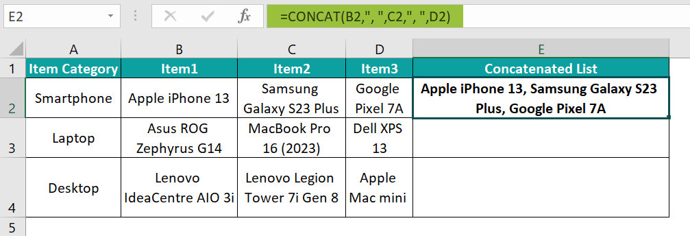
[ Alternatively, choose cell E2, and select Formulas → Text → CONCAT to open the Function Arguments window.
And update the mandatory and optional argument fields in the Function Arguments window.
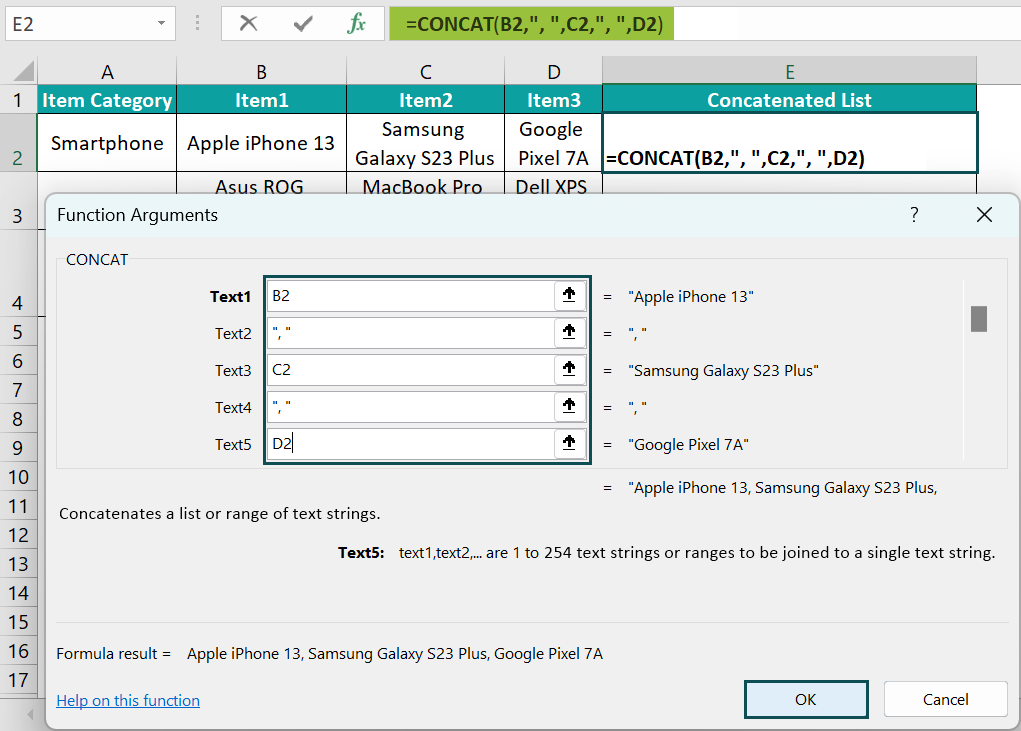
And click OK to obtain the required concatenated list for the Smartphone category in cell E2.]
- Step 3: Enter the formula in cells E3:E4 using the Excel fill handle.

The CONCAT() accepts five input values. And it combines them in the order specified in the formula.
Please note that we insert a space character after the comma within double quotes to ensure the result will show the specified text strings with a comma and space in between.
On the other hand, here is how we can use the TEXTJOIN() to concatenate the required strings in the target cells.
- Step 1: Choose cell E2, enter the TEXTJOIN(), as shown below:
=TEXTJOIN(“, “,

Next, once we enter the comma in the above formula, Excel will show an option to enter the second argument, ignore_empty, as TRUE or FALSE.
We can double-click on the required value based on whether we wish to ignore empty cells or include them when present in the source data.
In this case, we shall choose TRUE, followed by a comma.

And then, enter the given strings or references to cells containing the required strings to concatenate, separated by commas, and close the bracket.
=TEXTJOIN(“, “,TRUE,B2,C2,D2)

- Step 2: Press Enter to view the required concatenated list for the Smartphone category in cell E2.

[ Alternatively, choose cell E2, and select Formulas → Text → TEXTJOIN to open the Function Arguments window.
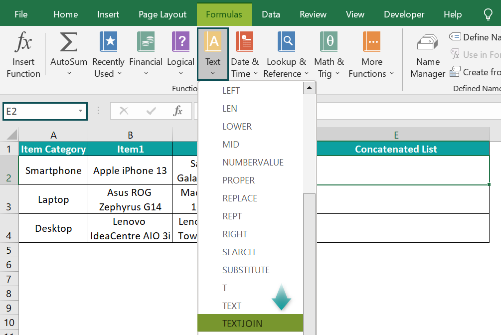
And update the mandatory and optional argument fields in the Function Arguments window.

And click OK to obtain the required concatenated list for the Smartphone category in cell E2.]
- Step 3: Enter the formula in cells E3:E4 using the fill handle.

The first argument in the TEXTJOIN() is the delimiter. And hence, we provide a comma and space character within double quotes for the same reason explained earlier.
Next, we enter the ignore_empty argument value as TRUE to ignore empty cells. And then, we can supply the text strings or cell references to the text strings, separated by commas, to the function.
And the function combines the specified text strings with the cited delimiter between them.
Example #2 – Use The Ampersand (&) Symbol As The Alternative
We can use the Ampersand symbol (‘&’) as an alternative to the CONCAT and TEXTJOIN functions.
Continuing with the above example, here is how to use the ‘&’ symbol to concatenate strings in Excel cells E2:E4.
- Step 1: Select cell E2 and enter the following formula.
=B2&”, “&C2&”, “&D2

- Step 2: Press Enter to execute the formula and obtain the following output.

- Step 3: Copy the formula in cell E3:E4 using the fill handle.

The ‘&’ symbol combines the input strings or cell references to strings and the separator in the order specified in the formula.
Example #3 – CONCATENATE Cell Values With Manual Values
We can combine cell values with manual values using the CONCAT().
For example, the table below lists top tech companies and their annual revenue for 2022-23.

And the requirement is to show the data as comments in column C.
Then, here is how to use the CONCAT() to combine the given values and text strings, entered manually, in the target cells to achieve the desired output.
- Step 1: Choose cell C2 and enter the CONCAT().
=CONCAT(A2,”‘s Annual Revenue (2022-23) is “,B2,”.”)

- Step 2: Press Enter to view the function output in cell C2.

- Step 3: Use the fill handle to update the formula in cells C3:C6.

In the above formula, the CONCAT() accepts two cell values from columns A and B, and we manually enter the required text strings within double quotes.
Thus, the CONCAT() joins the cell and the manual values in the same order as we supplied them as the argument values to the function in the above formula.
Please note that after the first argument value, the column A cell reference, the second argument is a text string within double quotes. But the string value starts with an apostrophe. So, the output shows the company name followed by an apostrophe without a space.
On the other hand, at the end of the string, supplied as the second argument value, there is a space character after the word “is”. And hence, the output shows a space between the word “is” and the column B cell value, the third argument value.
Also, the currency value contains the character “B”, indicating Billion. And that is why the CONCAT() displayed the currency value in the concatenated string in the same format as the source data.
But, if the currency value did not contain the character “B”, we must supply the currency value to the CONCAT() using the TEXT() as shown below.
TEXT(Value, “$#,##0.00_);[Red]($#,##0.00)”)
The reason is that the CONCAT() would show the currency value as a decimal number when supplying the currency value or cell reference to the currency value. But the above TEXT() expression will ensure the currency value gets displayed in the same format as the source data in the resulting concatenated string.
Furthermore, we can also use the CONCATENATE() in the target cells and obtain the above output.
- Step 1: Choose cell C2 and enter the CONCATENATE().
=CONCATENATE(A2,”‘s Annual Revenue (2022-23) is “,B2,”.”)

- Step 2: Press Enter to view the function output in cell C2.

- Step 3: Use the fill handle to update the formula in cells C3:C6.

Example #4 – CONCATENATE Date Values
We can concatenate date values using the methods explained in the section, How to do Excel String Concatenation?
For example, the table below shows the different phases of a short-term project, with their start and end dates.

And the requirement is to display the data as comments in column D.
Then, we can concatenate the given data using the ‘&’ symbol in the target cells, as shown below:
- Step 1: Select cell D2, enter the following ‘&’ symbol-based string concatenation formula, and press Enter.
=”The project phase, “&A2&”, starts on “&B2&” and ends on “&C2&”.”

And using the fill handle, update the formula in cells D3:D6.

However, the output shows the date values as their serial number equivalents.
So, we can use TEXT() to display the date values in the same format as the source data. And in this case, we use the TEXT() as we cannot perform any calculations using the date values in the resulting concatenated strings.
- Step 1: Choose cell D2, enter the following formula, and press Enter.
=”The project phase, “&A2&”, starts on “&TEXT(B2,”D-MMM-YY”)&” and ends on “&TEXT(C2,”D-MMM-YY”)&”.”

- Step 2: Using the fill handle, update the formula in cells D3:D6.

First, the TEXT() returns the input date value as a text in the specified format. And then, the ‘&’ symbol joins the text strings, provided in double quotes, cell values, and the TEXT() output in the same order as specified in the formula.
Further, cells A2, A3, and A5 contain the ‘&’ symbol. And they get displayed in the output. We can also supply the given text strings containing the ‘&’ symbol in double quotes and achieve the required output. The reason is that Excel does not consider the ‘&’ symbol as a concatenation operator when entered in double quotations.
Important Things To Note
- All the methods to concatenate strings in Excelare case-sensitive.
- For an invalid input string or cell value, the Excel string concatenation methods return the #VALUE! error.
- We must provide the delimiters and separators at the required positions while entering the CONCAT() and the Ampersand symbol-based string concatenation formulas. But, in the case of the TEXTJOIN(), we can provide the delimiter as the first argument to ensure it gets inserted between each input string in the resulting concatenated string.
- The CONCATENATE() was replaced by a more accurate function CONCAT in Excel 2016 version. However, the CONCATENATE() is still available as a Compatibility function under the More Functions group in the Formulas tab.

Frequently Asked Questions (FAQs)
We can concatenate strings in Excel VBA using the CELLS().
For example, the table below lists students’ first and last names.
And the requirement is to combine the students’ first and last names to display their full names in column C.
Then, here is how to concatenate the given strings using Excel VBA.
• Step 1: Open the source data worksheet and press Alt + F11 to open the VBA Editor.
• Step 2: Select the applicable VBAProject and choose the Insert tab → Module to open a new module window.

• Step 3: Click inside the module window and enter the VBA code to concatenate the text strings in the corresponding target cells.
• Step 4: Execute the code by clicking the play icon in the top menu.
Finally, open the active worksheet to view the output.
The VBA code contains a For loop, with the counter to count the row numbers.
And the CELLS()-based command inside the For loop concatenates the value in the cells, the coordinates for which the second and third CELLS() return, with a space in between.
And then, the resulting concatenated string gets assigned to a cell, the coordinates for which the first CELLS() returns.
Finally, in this way, each cell in the target cell range gets updated with the concatenated strings using the input text strings in the corresponding rows.
We can concatenate two strings in Excel with IF condition using the following steps:
1) Select a target cell and enter =IF(.
2) Enter the required IF condition and a comma.
3) Enter the CONCAT(), with the two given text strings supplied as the function argument values, if the requirement is to concatenate them for a TRUE IF condition. And enter a comma and the applicable FALSE value.
Otherwise, enter the applicable TRUE value, followed by a comma. And, enter the CONCAT(), with the two given text strings supplied as the function argument values, if the requirement is to concatenate them for a FALSE IF condition.
4) Finally, close the bracket and press Enter to view the IF() output as the two strings concatenated based on the specified IF condition.
We can concatenate string with double quotes in Excel using the following formulas:
=CONCAT(CHAR(34),text1,text2,….,CHAR(34))
Or
=CONCAT(“”””,text1,text2,….,””””)
The text1, text2,…. arguments are the text strings to concatenate. And entering the function CHAR(34) or double quotes within double quotes as the first and last argument values in the CONCAT() will show the concatenated string in double quotes.
Download Template
This article must be helpful to understand the Concatenate Strings In Excel, with its formula and examples. You can download the template here to use it instantly.
Recommended Articles
This has been a guide to What Is Concatenate Strings In Excel. We learn to concatenate strings using “&”, CONCAT, and TEXTJOIN with examples. You can learn more from the following articles –

Leave a Reply