What Is COUNTIF And COUNTIFS Function With Multiple Criteria?
The COUNTIF and COUNTIFS functions with Multiple Criteria checks the dataset based on the specified one or more condition, respectively, and returns the count of the cells that fulfill the criteria. The function helps us to check for Multiple Criteria in the same column or Multiple Criteria in multiple columns. The COUNTIF and COUNTIFS functions are inbuilt Statistical functions, so we can insert the formula from the “Function Library” or enter it directly in the worksheet.
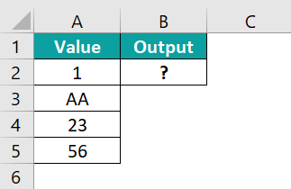
For example, in the following table, column A contains some values. We will count the cells that fulfill the specified condition using the COUNTIFS formula.
Select cell B2, enter the formula =COUNTIFS(A2:A5,“AA”), and press “Enter”.
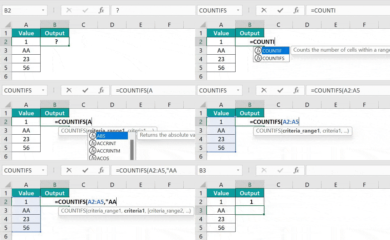
The output is shown above. The criteria is to find the count of cells with the value “AA”, within the cell range. Only one cell with that value matches the criteria, and so the count is 1.
Table of contents
- What Is COUNTIF And COUNTIFS Function With Multiple Criteria?
Key Takeaways
- Using the COUNTIF formula, users can count the cell matching the test condition or criteria. It is a Statistical Excel function.
- The second argument of the COUNTIF function is ‘Criteria,’ which is case insensitive.
- We can search the criteria for both numeric and alphabetic table arrays.
- The COUNTIF and COUNTIFS functions are almost the same. However, we must add or repeat the formula for the COUNTIF with Multiple Criteria, but add the cell ranges and the required criteria within the formula, separated by a comma, for the COUNTIFS with Multiple Criteria.
How To Use COUNTIF With Multiple Criteria?
The steps to use the COUNTIF with Multiple Criteria are as follows;
- Choose an empty cell for the output.
- Type =COUNTIF( select the cell range, enter the first criteria as a cell value or a reference, and close the brackets.
- Then press the “+”, and repeat step 2 with new values.
- Then press the “+”, and repeat step 2 with new values.
- The formula will be as per the syntax =COUNTIF(range,criteria)+COUNTIF(range,criteria), and finally, press “Enter”.
Examples Of COUNTIF With Multiple Criteria in Excel
We will understand some advanced scenarios with examples for the COUNTIF with Multiple Criteria.
Example #1
We will count the values using the COUNTIF with Multiple Criteria.
In the table, the data is,
- Column A shows the values.
- Column B will display the output.

The steps to count the number of cells using the COUNTIF with Multiple Criteria in excel are as follows:
- Step 1: Select cell B2, and enter the formula with the first cell range and the first criteria =COUNTIF(A2:A5,“A”)

- Step 2: In continuation with the formula, press the + sign, as shown below.

- Step 3: Now, enter the formula with the new cell range and the required criteria =COUNTIF(A2:A5,“B”). So the complete formula is =COUNTIF(A2:A5,”A”)+COUNTIF(A2:A5,”B”).

- Step 4: Finally, press “Enter”.

We get the output shown above. The count is 2, i.e., 2 cells matching the multiple criteria values A and B.
Example #2
We will count the values using the COUNTIF with Multiple Criteria.
In the table, the data is,
- Column A shows the values.
- Column B will display the output.

The steps to count the number of cells using the COUNTIF with Multiple Criteria are as follows:
- Step 1: Select cell B2, and enter the formula =COUNTIF(A2:A6,”Apple”)+COUNTIF(A2:A6,”Banana”).

- Step 2: Press “Enter”.

We get the output shown above. Here, there are 2 cells matching the 2 criteria, so the COUNTIF is 2.
Example #3
We will count the values using the COUNTIF with Multiple Criteria.
In the table, the data is,
- Column A shows the values.
- Column B will display the output.
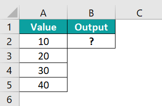
The steps to count the number of cells are as follows:
- Step 1: Select cell B2, and enter the formula =COUNTIF(A2:A5,”>20″)+COUNTIF(A2:A5,”<20″).

- Step 2: Press “Enter”.

We get the output shown above. Here, there are 3 cells matching the 2 criteria, so the COUNTIF is 3.
How To Use COUNTIFS Excel Function With Multiple Criteria?
The steps to use the COUNTIFS with Multiple Criteria are as follows:
- 1: Choose an empty cell for the output.
- 2: Type =COUNTIFS( and select the cell range and enter the first criteria, second cell range, next required criteria, and so on… as a cell value or a reference, and close the brackets.
- 3: The formula will be as per the syntax =COUNTIFS(criteria_range1,criteria1,[criteria_range2,criteria2],…), and finally, press “Enter”.
Examples Of COUNTIFS Excel Function With Multiple Criteria
We will understand some advanced scenarios with examples.
Example #1
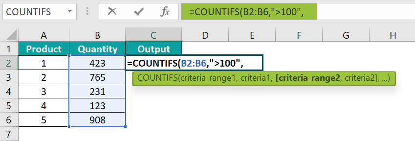
We will count the values using the COUNTIFS function With Multiple Criteria.
In the table, the data is,
- Column A shows the Product.
- Here, column B shows the quantity.
- Column C will display the output.
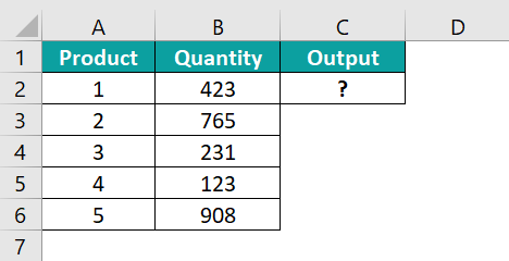
The steps to count the number of cells are as follows:
- Step 1: Select cell C2, and enter the formula =COUNTIFS(B2:B6,“>100”,
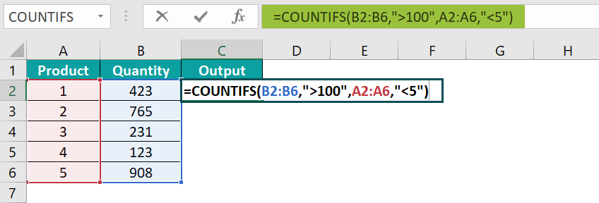
- Step 2: To continue the formula enter A2:A6,“<5” and close the brackets. So, the complete formula is =COUNTIFS(B2:B6,”>100″,A2:A6,”<5″)
- Step 3: Press the “Enter” key.
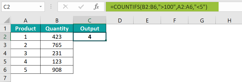
The output is ‘4’, as shown above. Here, there are 4 cells matching the 2 criteria, so the COUNTIFS is 4.
Example #2
We will count the values using the COUNTIFS function With Multiple Criteria.
In the table, the data is,
- Column A shows the Date.
- Column B will display the output.

The steps to count the number of cells are as follows:
- Step 1: Select cell B2, and enter the formula =COUNTIFS(A2:A5,”>01-12-2019″,A2:A5,”<19-01-2022″)

- Step 2: Press the “Enter” key.

The output is ‘2’, as shown above. Here, there are 2 cells matching the 2 criteria, so the COUNTIFS is 2.
Example #3
We will count the values using the COUNTIFS function With Multiple Criteria.
In the table, the data is,
- Column A shows the Product.
- Here, column B shows the Status.
- Column C will display the output.

The steps to count the number of cells are as follows:
- Step 1: Select cell C2, and enter the formula =COUNTIFS(B2:B6,”Delivered”,A2:A6,”Milk”)

- Step 2: Press the “Enter” key.

The output is ‘1’, as shown above. Here, there is 1 cell matching the 2 criteria, so the COUNTIFS is 1.
Important Things To Note
- There are five variants of the COUNT function group. They are COUNT Excel funciton, COUNTA, COUNTIF, COUNTIFS, and COUNTBLANK.
- The #VALUE! error occurs when text passed in the criteria has more than 255 characters in length.
- In the ‘Criteria’ argument of the syntaxes of the COUNTIF and COUNTIFS functions, the special characters ‘? (Question mark) matches any one characterand * (Asterisk)’ matches a series of characters that are in a sequence.

Frequently Asked Questions (FAQs)
The COUNTIF function and COUNTIFS function are from the COUNT function group, like the COUNTA and COUNTBLANK functions. It is the predefined function in Excel. It counts all the cells in the range specified by the single or multiple conditions.
• The formula of the COUNTIF function is =COUNTIF(range,criteria)
• The formula of the COUNTIF function for multiple criteria is =COUNTIF(range,criteria)+ COUNTIF(range,criteria)+ COUNTIF(range,criteria)+ and so on…
• The formula of the COUNTIFS function is =COUNTIFS(range1,criteria1,[criteria_range2,criteria2],…)
The COUNTIF Excel function with multiple criteria is used to count cells in a cell range matching a single criteria together with multiple cell ranges with 2 or more conditions.
The COUNTIF function in Excel is in the Formulas tab, we can insert it as follows:
First, choose an empty cell → select the “Formulas” tab → go to the “Function Library” group → click the “More Functions” option drop-down → go to the “Statistical” option and click the right arrow → select the “COUNTIF” function, as shown below.
Download Template
This article must help understand the COUNTIF With Multiple Criteria, formulas, and examples. You can download the template here to use it instantly.
Recommended Articles
This has been a guide to COUNTIF With Multiple Criteria in Excel. Here we use the COUNTIF & COUNTIFS formulas with multiple criteria, examples & downloadable excel template. You can learn more from the following articles –

Leave a Reply