
What Is COUNTIFS Function In Google Sheets?
The COUNTIFS function in Google Sheets helps users find the count of the selected values by taking multiple criteria into consideration.
The Google Sheets COUNTIFS function is a combination of the COUNT and the IFS functions. Hence, the function will count the values based on the provided criteria or conditions. The advantage with the function is that it can take multiple criteria.
Use this COUNTIFS Function In Google Sheets Template to follow along with the examples in this article.
Download Excel TemplateFor example, the following data consists of different items and their quantity for the months, January to March. We will use the COUNTIFS to check for two criterias.

Select cell E2, enter the formula =countifs(A2:A10,”Mar”,B2:B10,”C”) and press “Enter”, as shown below.

The result is 1, because the formula checks for the two scenarios that the first cell range is “Mar” and the second cell range is item “C”. We see that only one row, i.e., row 10, satisfies both criterias.
Key Takeaways
- The COUNTIFS function in Google Sheets looks for multiple criteria and returns count only from the matching criteria that satisfies or fulfills all the criterias given in the formula.
- The function takes the criteria reference in the form of Text, Number, Date, and all the logical operators, however, ensure to insert the same within double-quotes (“ ”) orif it is a pair, then, within flower brackets “{}”.
- If we want to count withing the same range, then, we must choose the cell range twice and use the logical operators
- If we are giving the date as the criteria, we need to give the logical operators in double quotes and then concatenate the date using the ampersand (&) symbol.
COUNTIFS() Google Sheets Formula
The syntax of the COUNTIFS Google Sheets Formula is,

The arguments of the COUNTIFS Google Sheets Formula are,
- criteria_range1: It is the first criteria range in which criterion1 will be evaluated. It is a mandatory argument.
- criterion1: It is the first condition that is checked which is entered as a text in double-quotes, irrespective of the values such as, number, cell reference or any other Google Sheets function input. It is a mandatory argument.
- [criteria_range2, criteria_range3, criteria_range4 and so on…]: It is an optional argument. Here, we must select the second criteria range in where the criterion2 will be evaluated.
- [criterion2, criterion3, criterion4 and so on…]: It is an optional argument. We can supply the second condition to be considered within the criteria range 2.
How To Use COUNTIFS Google Sheets Function?
We can use the COUNTIFS In Google Sheets in 2 ways, namely,
- Access from the Google Sheets ribbon.
- Enter in the worksheet manually.
Method #1 – Access from the Google Sheets ribbon –
Choose an empty cell for the output – select the “Insert” tab – click the “Function” option right arrow – click the “Math” option right arrow – select the “COUNTIFS” function, as shown below.

The “COUNTIFS” formula appears, as shown below. Enter the argument as the cell reference.

Method #2 – Enter in the worksheet manually –
- Select an empty cell to display the output.
- Type =COUNTIFS( in the selected cell. Alternatively, type =C or =COUNT and double-click the COUNTIFS function from the list of suggestions shown by Google Sheets.
- Enter the arguments as cell references or cell range.
- Close the parenthesis and press the Enter key.
Examples
Let us consider some examples to understand the COUNTIFS Google Sheets function for three conditions, for date values, for logical operators and with just one column cell range.
Example #1 – Three Conditions (Multiple Criteria)
The following data consists of the fruits, their categories and the order dates. We will count the cells that satisfy three criterias.

The procedure to find the count of values that satisfy three criterias using the COUNTIFS is,
Select cell A14 and enter the formula =COUNTIFS(A2:A11,”Banana”,B2:B11,”3″,C2:C11,”12-Jun-2023″)

Then, press “Enter”. We get the output shown below.

The result is 1. The formula checks for the three scenarios, 1st cell range is “Banana”, 2nd cell range is category “3” and 3rd cell range is dated 12-Jun-2023. We see that only one row, i.e., row 7, satisfies the three criterias.
Example #2 – Using COUNTIFS with Date Criteria
The following data consists of date values. We will count the dates that fall within a specified date. The COUNTIFS function will allow us to apply logical operators to get the count between two dates.

The procedure to find the count of date values between two dates using the COUNTIFS is,
Select cell C4 and enter the formula =COUNTIFS(A2:A11,”>10-Jun-2023″,A2:A11,”<14-Jun-2023″).

Then, press “Enter”. We get the output shown below.

The result is 5. The formula checks for the two scenarios in the same cell range, where the dates are “>10-Jun-2023” and “<14-Jun-2023”. We see that five dates values in the cells A4:A8, fall between the two dates.
Example #3 – Using COUNTIFS with Logical Operators
COUNTIFS function’s versatility is that we can use all kinds of logical operators to apply the criteria. The following logical operators in Google Sheets are commonly used with the COUNTIFS function.
- Greater Than.
- >= Greater Than or Equal to.
- < Less Than.
- <= Less Than or Equal to.
- = Equal to.
- <> Not Equal to.
The data given below consists of some products with their number of units sold. We will find the count of the values that satisfy the criterias using the logical operators with the COUNTIFS function.

The procedure to find the count of date values between two dates using the COUNTIFS is,
Select cell C2 and enter the formula =COUNTIFS(B2:B11,”>500″,A2:A11,”<>Laptops”)
Then, press “Enter”. We get the output shown below.

Then, press “Enter”. We get the output shown below.

The result is 3, as the formula checks for two scenarios, 1st cell range is “>500” and 2nd cell range is not a laptop, i.e., “<>Laptop”. We see that the cells A6, A10 and A11 satisfy the given criterias.
Example #4 – Using COUNTIFS to Count Cells in the Same Column
The data below consists of the four metropolitan cities. We will use the “ArrayFormula + Sum + Countifs” to Count the cells in the Same Column by giving the criterion values in pairs.

The steps to count cells in the same column are as follows:
Step 1: Select cell C6 and enter the formula =sum(COUNTIFS(A2:A13,{“Delhi”,”Kolkata”})), as shown below.
[Note: The flower brackets “{}” is inserted because we are using the criterion argument in pairs.}

Step 2: Now, execute the formula as an array formula. Therefore, press “Ctrl+Shift+Enter”, then, the formula becomes =ArrayFormula(sum(COUNTIFS(A2:A13,{“Delhi”,”Kolkata”})))

Step 3: Finally, press “Enter” to get the output shown below.

The result is 6, as the formula checks for two scenarios in the same cell range, if the criterion is “Delhi + Kolkata”. Then, it adds the total and returns the same.
COUNTIF vs COUNTIFS
A few differences of COUNTIF & COUNTIFS are as follows:
- The COUNTIF takes only one criterion, but COUNTIFS takes multiple criterias.
- The COUNTIF takes one criterion and gives the exact match or partial match. Whereas, the COUTNIFS function looks for the exact match of the criteria in the given range. If the criteria given are not exact, then it will return the count as 0.
Important Things To Note
- The COUNTIFS function will return #VALUE! error when the criteria range selection is not consistent.
- When we supply the date criteria, the date value should be in the same format as in the data range.
Frequently Asked Questions (FAQs)
We often forget in which category a function falls, here, the “COUNTIFS” function. Then, we can insert the function as follows:
Choose an empty cell – select the “Insert” tab – click the “Function” option right arrow – click the “All” option right arrow – select the “COUNTIFS” function, as shown below.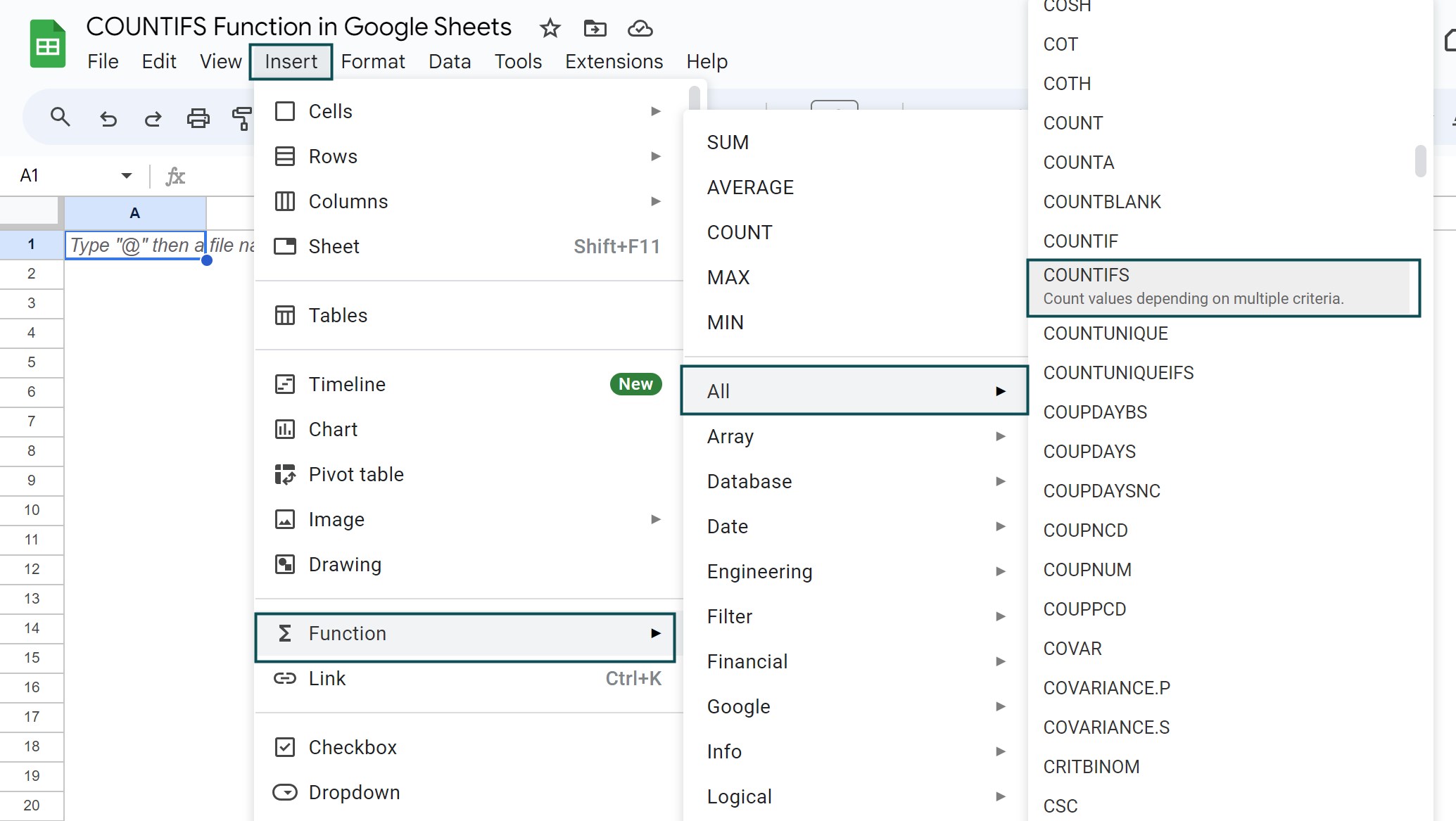
However, as always, entering the function manually is the best way to avoid confusion.
Alternatively, we can find the Functions icon to insert the COUNTIFS function by following the path shown below.
Choose an empty cell – click the “More” option represented by the three vertical dots at the end of the toolbar, as shown below.
A list of icons appears when we click the “More” option. Here, click the “Functions” icon, as shown below.
Here, click the “Functions” option – click the “All” option right arrow – select the “COUNTIFS” function, as shown below.
A few reasons the COUNTIFS function may not work are,
a. The required criteria range selection must be the same across multiple range selection and the criteria value should be the exact match in the criteria range.
b. We have not entered the criterion argument as textual values, i.e. it is not entered in double-quotes.
c. The entered data range does not exist or is deleted.
Use this COUNTIFS Function In Google Sheets Template to follow along with the examples in this article.
Download Excel Template