Data Bars in Excel

What is Data Bars in Excel?

Data bars in Excel are a type of conditional formatting that visually represent the presented data. They are colored bars added to cells to compare their values. Larger the value, the longer the bar. They are beneficial as a visual representation tool for the comparison of values.

Below is a table containing some books’ names and the number of copies sold in a bookstore. Here, we can apply data bars in Excel to compare the sales details and find the best-selling books. For it, go to the Home tab, click on the Conditional Formatting option, and choose Data Bars. You can select any data bar according to your requirements. Thus, you can find the best-selling book immediately.

Explanation and Uses

Data bars in Excel are a cool feature that visually shows the relationship between data. It makes your worksheet easier to understand.
Data bars can only measure quantitative values. Apart from numbers, we cannot apply conditional formatting with data bars to cells with text or blank cells.
They are in the exact location of the data, unlike bar charts.
They are helpful for values that are closer to each other.
You can set different rules for formatting them, like formatting only the top and bottom values, formatting unique values, and so on. You can also customize the color, the fill, the border, and other features.
Data bars in Excel can also be used to show negative values.
The bars appear from the left side of the cell towards the right for positive numbers and gravitate toward the left for negative numbers. In the case of mixed values, the center is adjusted to accommodate both types of bars.

What is Data Bars in Excel?

Data bars in Excel provide a graphical representation of the values in a cell/range of cells making it easy to compare them. They can be easily added by choosing the Home tab and then Conditional Formatting.
There are two kinds of Data Bars you can display; one is the Gradient Fill, and the other is Solid fill.
You can change the color of the bar under the option Manage Rule and display both positive and negative bars in different colors.

How to Add Data Bars in Excel?

Data Bars in Excel are convenient; the good news is that they are effortless to use! Let us look at an example where we have the top goal scorers of the football World Cup, 2022. To represent the data visually and find the top scorer, try inserting data bars in Excel.

We must apply the data bars to the column “Goals.” Select the cell range from C2 to C9. Next, go to Home tab and click on Conditional Formatting from the Styles group.
In the drop-down list, select the Data bars option and choose from either Gradient or Solid fill.
We have selected Gradient fill. Notice how the bars are used to represent the different values.

Looking at this image, we can easily find the highest goal scorer, Mbappe.
You can also use Data Bars based on specific conditions. When you go to the option Data Bars under Conditional Formatting, choose the option for More Rules; you get a pop-up window.
You can apply any formatting rule.
• We have chosen the option “Format only Top and Bottom ranked values.”
• We have set formatting only the Top 2 values.
• Click on the button “Format” and put any formatting requirements.
• We have chosen to highlight the Top 2 values in Purple with a double underline option.

Thus, you can see that the top 2 ranked values have been formatted as specified.

Examples

Below, we present some examples of how data bars are helpful for the conditional formatting of cells with numbers.

Example #1

Set Data Bar Minimum and Maximum Value

Let us enter the scores of some students in a class. But first, we must add Data Bars to provide a graphical representation and highlight the values in the table and how they are related.

Step 1: Select the cells from B2 to B8 to add Data bars. Go to the option Conditional Formatting in the Home tab. Click on Data Bars. You can choose from the range of colors available and the Solid or Gradient fill.

Step 2: We have chosen the option Gradient Fill and the red color. Observe the result.

We have the longest bar for the score of 99 in cell B5. Here, notice how the bar for the least score 23 is not at the beginning of the cell but some way off. Now, we can set the maximum and minimum values for the data bars representation.

Step 3: After selecting the cell range from B2 to B8, choose the Conditional Formatting option and choose More Rules.

Step 4: In the pop-up window, choose “Number” under the Minimum and Maximum options. Enter the minimum and maximum values for the bars.

Step 5: Press OK. Now, check the Data Bars. You can see how the bar sizes have changed according to the Maximum and Minimum values.

Data Bars in Excel - Example 1 - Step 5a

Here, we have a comparison of the data bars before and after applying the maximum and minimum values. Notice the bars in B3 and B5.

Data Bars in Excel - Example 1 - Step 5b

Example #2

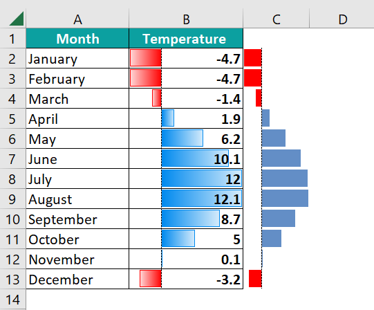
In this example, we will look at how negative values are represented using Data Bars. Now, for example, we have the average monthly temperature of a city in the table below. Let us define the temperature with conditional formatting data bars in Excel.

Step 1: Go to the Conditional Formatting and click on Data Bars. We have chosen the Light Blue Data Bar option.

Step 2: You get the Data Bars as shown below. Let’s try to copy this bar outside Excel.

Step 3: To copy the bars outside Excel. Go to cell C2 and type =B2. Press Enter and drag the handle from C2 to C13. All the values in B2 get copied into the corresponding cells in C2.

Step 4: Now, select the cells from C2 to C13 and choose the Data bars option in Conditional formatting.
- Select the required Data bar colors and type.
- Now go to the “More Rules” option.
- In the pop-up window, enable the checkbox for Show Bar Only. Click OK.

You get only the colored bars in the next column.

Step 5: Thus, the Data Bars can also be represented outside the cell, as shown above. Now, how to delete the bars in Column B?

Select cells B2 to B13. Go to Manage Rules under Conditional Formatting.

Step 6: Select the rule applied and click on Delete Rule. Press OK.

The data bars in Column B are deleted.

Data Bars in Excel - Example 2 - Step 6b

Example #3

We have the details of the number of cars sold by a dealer in different cities over 5 months. We can set certain conditions and use data bars. Let us format data bars in Excel to find those cities which have sold more than 50 cars.

Step 1: Let us set the conditions for the same. Go to Conditional Formatting and select Data Bars. Select the “More Rules” option here. You will get a pop-up window.

Step 2: As seen above, set the type to Number for Minimum and Maximum. Enter the maximum and minimum values you want to set. Press OK.

You can see that the data bars have been applied for those numbers above 50.

Therefore, we can immediately track all those cities which sold above 50 cars and the month in which they were sold. It gives you an idea of where to improve your sales and the months to concentrate.

Important Things to Note

Data bars can be applied for values and not the text format.
You can apply data bars to a cell, cell range, table, or whole worksheet.
In Excel, data bars represent a wide range of negative and positive data values. If your cell range contains positive and negative values, the data bars are changed to represent these values in different colors.
It works only through one axis, which is the horizontal axis.

Frequently Asked Questions (FAQs)

1. How to add solid fill data bars in Excel?

You should select the required cell range. Then, go to Home tab and click on Conditional Formatting. Next, select the Data bars option in the drop-down list and choose Solid fill.

2. How to remove Data bars in Excel?

Select the range to remove the data bars and go to Conditional Formatting in the Home tab. Next, click on the option Clear Rules, and select either the “Clear Rules from Entire Sheet” or “Clear Rules from Selected Cells” option. You can also click on the Manage Rules option, select the required rule and press Delete Rule.

3. Why is data bars in Excel not working?

Data bars in Excel work only for numbers or quantitative data. If the data is in text format, the application of data bars will not work. The data bars will also not work for empty cells.

4. How to set maximum length of data bars in Excel?

After selecting the cell range:
1) Go to Conditional Formatting and choose More Rules.
2) In the popup window, choose “Number” under the Maximum option.
3) Enter the maximum value and press OK.

Download Template

This article must help understand the Data Bars in Excel, its features and examples. You can download the template here to use it instantly.

Data Bars in Excel Download