DGET in Google Sheets

What is DGET in Google Sheets?

The DGET function in Google Sheets can be used to extract a single value from a database that matches specific criteria. The function looks through a range and checks which rows meet the given conditions. It then returns the value from a specified column.

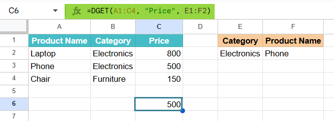
DGET is very useful when working with datasets where you want to pull out a unique value based on one or more criteria. It is like having a lookup function. However, if more than one record matches the condition, you will get an error with DGET. This is because it is designed to return only one unique result. For example, suppose there is a product list in Google Sheets with columns for Product Name, Category, and Price. If we wish to find the price of a product in a specific category that meets certain criteria, we can use DGET to quickly retrieve that value. For this, enter the following formula:

=DGET(A1:C4, “Price”, E1:F2).

Here, we get the result 500, which is the price of the  Phone in the Electronics category. Look at how the database has been provided.

Syntax

Now that we have a brief grasp of what DGET does, let’s look at the DGET in Google Sheets formula for the function:

=DGET(database, field, criteria)

Arguments meaning:

• database – The range of cells that make up the database. The first row should contain the column labels.
• field – The column from which to return the value. You can enter this as the column label in quotes (e.g., “Price”) or as a column number (e.g., 3).
• criteria – The range containing the condition to match. This range must include at least one column label and one cell containing the condition.

How To Use DGET Function in Google Sheets?

The DGET function is used to retrieve a specific value from a database range based on some given conditions. It is a very powerful and is used when we have to work with structured data. The database should also include column headers. You can use DGET to filter out any unique information such as an employee’s salary, a product’s price, or a student’s score which matches a defined criterion.

You can use the DGET function in two ways:

• By manually typing DGET
• By selecting it from the Google Sheets menu

Using DGET Function Manually

Now, we want to find the Price of the Phone in the Electronics category. As we have seen before, we got the price of the Phone in the Electronics category.

Step 1: In cells E1 to F2, we enter the following details.

Step 2: Now, we enter the DGET formula. Click on an empty cell and type the following formula:

=DGET(A1:C5, “Price”, E1:F2). The arguments are within parentheses and separated by commas.

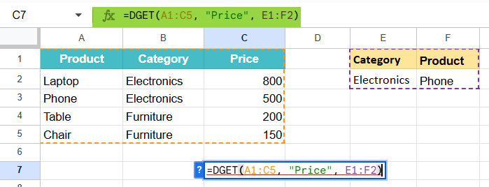
Step 3: Press Enter. The cell will display 500, which is the price of the Phone in the Electronics category.

Using DGET From the Menu

1. Click on any empty cell.
2. Go to Insert → Function → Database → DGET.
3. In the function box, specify the database, field, and criteria.
4. Press Enter to see the result.

Examples

Let us look at some interesting examples to understand in detail how the DGET function works in Google Sheets.

Example #1 – Pull an Employee’s Salary Based on Their Name

In a company, the HR department regularly has to look up individual employee details. This includes details like salary or department. For this, they have a staff database. Instead of manually filtering or scrolling through many rows, they wish to find a quick way to retrieve an employee’s salary by entering their name. This improves both the accuracy and speed. The DGET function provides a easy way by allowing HR to pull precise data based on a simple search criterion.

Step 1: Open a Google Sheet and enter the following data in cells A1 to C6.

Step 2: In another part of the sheet, cells E1:F2, create a criteria range as shown below:

Step 3: Click on an empty cell and type the following formula:

=DGET(A1:C6, “Salary ($)”, E1:F2)

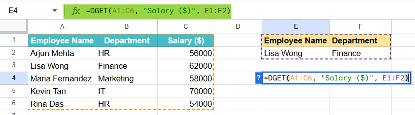
Step 4: Press Enter. The cell will display the result as 70000, which is Kevin Tan’s salary.

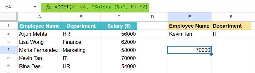
Step 5: To check how the formula works, change the employee’s name in the criteria table to “Lisa Wong” and the department to “Finance.”. Now check the result. It will automatically update to 62000.

Using DGET, the HR team can instantly retrieve any employee’s salary by simply changing the name in the criteria range. This makes payroll verification, salary audits, or individual lookups effortless and eliminates the need for complex filtering or manual searches.

Example #2

In this example, a university’s academic office tracks student grades across multiple subjects. The staff present must extract grades for a list of students without manually entering multiple formulas. To streamline this process, one can use DGET in Google Sheets. This enables them to perform multiple lookups automatically in one go.

Step 1: Enter the following dataset in cells A1 to C6.

Step 2: In cells E1 to E2, write the student’s name whose grades we may need.

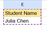
Step 3: In cell F1, enter the following formula:

= DGET(A1:C6, “Grade”, E1:E2)

Step 4: Press Enter. The formula retrieves the corresponding grade of that student.

Using DGET, administrators can pull multiple student grades at once, saving time and reducing human error. This approach scales efficiently for larger datasets, such as entire class reports or grade lists.

Example #3 – Using DGET with IF Function

We take another interesting example where a regional sales company wants to monitor whether each salesperson meets their monthly revenue targets. Instead of manually comparing the sales values, the manager wants a quick way to check and display whether the target has been achieved or not. By pairing DGET with the IF function, the manager can automatically evaluate, and label performance results based on each salesperson’s data.

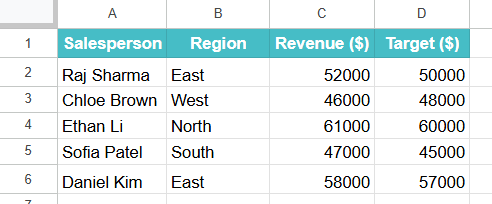
Step 1: Enter the following details of the employees in cells A1 to D6.

Step 2: Create a criteria range in E1:F2 as shown below:

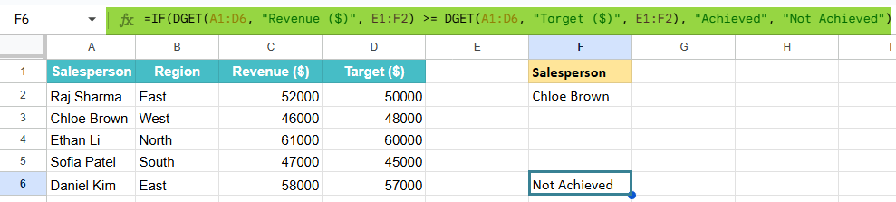
Step 3: In cell G1, enter the following formula:

=IF(DGET(A1:D6, “Revenue ($)”, E1:F2) >= DGET(A1:D6, “Target ($)”, E1:F2), “Achieved”, “Not Achieved”)

Step 4: Press Enter. The result will display “Not Achieved” because Chloe Brown’s revenue is less than her target of $48,000.

By combining DGET with IF, we get a formula that creates automatically evaluates performance vs Target and instantly flags performance results. This will help managers can easily assess targets and maintain an updated, data-driven performance dashboard without complex formulas.

Important Things to Note

1. If more than one record matches the given criteria, the function will return a #NUM! error. This is because the function is designed to retrieve a single value not multiple matches.
2. The first row of the range must contain the column labels because DGET uses these headers to identify fields and match them with the given criteria.
3. Whenever you specify conditions, ensure that the criteria range contains the same header names as the database.
4. You can specify the column to return from either by using the column label in quotes (e.g., “Price”) or the column index number (e.g., 3).
5. If no record meets the condition, DGET returns a #VALUE! error. Ensure your criteria are accurate and correspond to the database headers exactly.

Frequently Asked Questions (FAQs)

Download Template

This article must help understand the DGET Function in Google Sheets, with its formula and examples. We can download the template here to use it instantly.

Recommended Articles

Guide to What Is DGET Function In Google Sheets. We explain how to use the DGET Function In Google Sheets with examples and points to remember. You can learn more from the following articles. –

TOCOL in Google Sheets

VDB in Google Sheets

SYD in Google Sheets