
What is SYD in Google Sheets?
SYD is a function in Google Sheets that calculates the depreciation of an asset using the sum-of-years’-digits (SYD) method. This method considers an asset’s accelerated depreciation. Here, an asset’s value decreases more rapidly in its initial years of life. The function requires four arguments: cost (initial cost), salvage (the asset’s value at the end of its useful life), life (the total number of depreciation periods), and period (the specific period for which we must calculate depreciation).
For instance, a person has an asset that cost $10,000. It’s salvage value is $500, with a useful life of 5 years. Let us calculate its depreciation for the 3rd year using the formula:
=SYD(10000, 500, 5, 3)
We get the depreciation at the end of three years as $1,900. This is a simple method that makes it easy to calculate accelerated depreciation accurately with just a simple formula.

Use this SYD in Google Sheets Template to follow along with the examples in this article.
Download Excel TemplateKey Takeaways
- SYD in Google Sheets calculates the depreciation of an asset using the sum-of-years’ digits method, which accelerates expense recognition.
- The function is useful when assets lose value faster in the early years, such as vehicles, machinery, or technology equipment.
- The syntax of the SYD function is as follows:
=SYD(cost, salvage, life, period)
- SYD computes depreciation for a specific period, for e.g., Year 1, Year 2, and so on, rather than cumulative depreciation.
- If you need straight-line depreciation, use SLN; if you need double-declining balance.
Syntax
The SYD function in Google Sheets formula is as follows:
=SYD(cost, salvage, life, period)
Arguments are:
- cost: The initial cost of the asset.
- salvage: The value of the asset at the end of its useful life.
- life: The number of periods over which the asset will be depreciated.
- period: The specific period within the asset’s life for which to calculate depreciation.
How To Use SYD Function in Google Sheets?
The SYD function in Google Sheets is used to calculate the sum-of-years’ digits depreciation of an asset for a specified period. This method accelerates depreciation, meaning higher depreciation in earlier years and lower depreciation in the later years.
It is useful in scenarios where companies want to account for an asset losing more value in its initial years like specific machinery and tech equipment.
To enter the SYD function in Google Sheets, there are two main ways:
- Enter SYD manually
- From the Google Sheets menu
Enter SYD Manually
Let us look at the manual method to enter the SYD function. To illustrate this, we will calculate the depreciation of a machine with the following details:
- Initial Cost: $12,000
- Salvage Value: $1,000
- Useful Life: 5 years
We will calculate the depreciation for the first year.
Step 1: Open Google Sheets and in a new spreadsheet, enter the required details.

Step 2: Enter the SYD formula: in an empty cell B5. Here, we start with an = sign, followed by the function name and open braces. Enter the arguments in the order specified in the syntax, separated by a comma and close the braces.
=SYD(B1, B2, B3, B4)

Step 3: Press Enter. The cell B5 will display the depreciation amount for the first year, which is $3,666.67.

The result, $3,666.67, represents the depreciation expense for the machine during its first year of operation using the Sum of Years’ Digits method. To calculate depreciation for subsequent years, one must change the period argument accordingly (e.g., 2 for the second year, 3 for the third, and so on).
Entering SYD Through the Menu Bar
- Go to the Insert tab. Choose Function → Financial.
- From the list, select SYD.
- A tooltip will appear asking for four arguments.
- Fill them in with the proper values.
- Press Enter to get the result.
Examples
The primary purpose of SYD in Google Sheets is to calculate the sum-of-years’ digits depreciation for an asset over its useful life. Let us look at a simple example to do the same.
Example #1 – Calculate SYD for an automobile for $41,000, expect it to last 5 years, and trade it in for $4,000
Ley us use the SYD function to calculate accelerated depreciation of a automobile. For instance, let’s say you purchase an automobile for $41,000, expect it to last 5 years, and trade it in for $4,000. We want to calculate the depreciation for Year 1 using SYD.
Step 1: Set up your dataset with the following details in an empty spreadsheet.

Step 2: Let us enter the following formula.
=SYD(B1, B2, B3, B4)
Here:
- B1 → Cost of the automobile
- B2 → Salvage value after 5 years
- B3 → Life in years
- B4 → Period (year 1)

Step 3: Press Enter. We get the result as $20,000.00 depreciation for Year 1.

The automobile depreciates by $20,000 in Year 1 using the sum-of-years’ digits method.
Example #2 – Calculate SYD for a printing machine for $24,000, expect it to last 10 years, and trade it in for $3,000
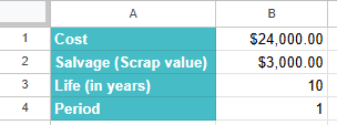
A person bought a printing machine for $24,000 that they expect to use for 10 years. At the end of its useful life, it is estimated to be traded in for $3,000. Let us calculate the depreciation to record in Year 1 using the sum-of-years’ digits (SYD) method.
Step 1: Set up the dataset. In an empty spreadsheet, enter the following details.
Create two columns (labels in column A, values in column B). Enter the machine’s cost, the expected salvage (trade-in) value, the useful life in years, and the period you’re calculating (Year 1).
Step 2: Enter the SYD formula. Click an empty cell where you want the result and type the formula using the cell references.
=SYD(B1, B2, B3, B4)

In this formula, the cost is B1), B2 is Salvage, B3 is Life, and B4 is Period. The SYD function uses the depreciable base (cost − salvage) and the “sum of years” denominator to compute the accelerated depreciation for the specified period.
Step 3: Press Enter. The cell will show the depreciation amount for Year 1. Internally the calculation is:
Using SYD, the printing machine’s depreciation for Year 1 is $3,818.18, reflecting accelerated expense recognition early in the asset’s life. This method is useful when an asset loses value faster in its initial years and you want accounting that matches that economic reality.

Example #3 –
To understand the uses of the SYD function better, let’s consider another example. Suppose we want to calculate the depreciation for an asset with an initial cost of $300,000 and a salvage value of $5,000 after 10 years. We need to calculate the depreciation over five years. The formula for calculating the depreciation amount will be as shown below:
Step 1: Enter all the details in a Google sheet.

Step 2: Enter the formula for depreciation in Year 1 as shown below. This is entered into cell C4. Press Enter.
=SYD(B1,B2,B3,B4)

Step 3: For the subsequent years, we will change the per argument.
So, for the second year, the formula would be =SYD(B1,B2,B3,B5). For the third year, the formula would be =SYD(B1,B2,B3,B6) and so on.
The result we get is shown below:

Important Things to Note
- The arguments life and period should be provided in the same units of time: days, months, or years.
- The SYD function is practical in many ways as it reflects how assets like machinery or tech equipment lose value more quickly at the beginning of their life cycle.
- Unlike some depreciation methods that give cumulative results, SYD focuses on depreciation for a specific year (or period), making it easy to build a year-by-year depreciation schedule.
Frequently Asked Questions (FAQs)
SYD is very useful because it provides a more accurate reflection of an asset’s depreciation. Many assets depreciate faster in the earlier years of their life, and they lose value more rapidly. This method of calculation can help businesses match their expenses better with the revenues generated by the assets.
Some of the common errors one would encounter include:
#VALUE! error – Occurs when any of the arguments are non-numeric.
#NUM! error – Occurs under the following circumstances:
The life or period argument is less than or equal to zero.
The salvage argument is less than zero.
The period argument is greater than the life argument provided.
SYD (Sum-of-Years’ Digits) gives accelerated depreciation but gradually decreases year by year.
SLN (Straight-Line) spreads depreciation evenly across all periods.
DDB (Double Declining Balance) applies a constant rate to the declining book value, resulting in very high depreciation at the start and smaller values later. SYD is often preferred when you want accelerated depreciation but with smoother reduction than DDB.
Use this SYD in Google Sheets Template to follow along with the examples in this article.
Download Excel TemplateRecommended Articles
Continue with these related resources when you want the next practical step in this topic.
- PV in Google Sheets
- FV in Google Sheets
- NPV in Google Sheets
- IRR Google Sheets Function
- PMT in Google Sheets
Explore the full Google Sheets Financial Functions guide or browse Google Sheets Resources.